DUCKDB Benchmarking
Data Intellect
Introduction
1. SELECT MAX(bsize) from quote
This query returns the maximum bsize (the size of the bid) within the quote table. Max is often a useful statistic, in this case the max bid could be used to analyse the best times to sell a particular asset.
2.“SELECT * FROM trade WHERE sym in (‘AIW’,’AUSF’,’BBDO’,’BDR’)”
Our second query also yields a small return (each sym appears only once within the trade table), and this time testing the ability of DuckDB to heavily filter the data.
3. “SELECT * FROM quote WHERE sym in (‘AAPL’)”
A relatively large return (600,000 rows), testing the ability of DuckDB to retrieve and format a relatively large set of data.
4. “SELECT sym, AVG(price) AS AvgPrice FROM trade GROUP BY sym”
A basic grouping, with a simple aggregation, one that is common within a lot of analytics.
5. “SELECT sym, MAX(price) AS maxprice, MIN(price) AS minprice FROM trade WHERE sym LIKE ‘A%’ GROUP BY sym”
A more complex set of aggregations with a filter performed first, as well as a grouping clause.
6. “SELECT sym, avg(price) AS AvgPrice FROM trade GROUP BY sym HAVING avg(price)>230”
Another aggregation but this time with a filter being performed after, changing this order makes a difference as we have to use all the data to perform the aggregation.
At this point we should probably highlight that the data we used was the NYSE TAQ data from October 2019. Due to the sheer size of this dataset, we took only the data between 3 and 4 o’clock, and for the quotes, we took only the syms beginning with ‘A’. This leaves us with trade and quote tables of 10 million and 1 million rows respectively.
A Detour into Shortcuts
We have changed our approach to timings since our last blog. For the millions who have read it, you may remember that when we were analyzing the time for the as-of join to complete, we came across a stumbling block in that, when we timed the query, the output was unthinkably fast (around 90 microseconds), therefore, we forced all the data to materialise by converting it to a pandas dataframe using .df() at the end of the query. Since our last blog, we have come to more of an understanding for the super-speed of DuckDB; laziness!
Doesn’t quite add up does it? Laziness causing speed. Within DuckDB, once connected to a database, there are three ways to call a query, con.query, con.sql and con.execute (within the Python API). The first two are relations, and within DuckDB, relations are lazy, this means that they cut corners by outputting only a snapshot of the data, and only executes the query on this data. Therefore, relations are really helpful for when you don’t want to return all the data to the console. But when it comes to timing queries, it’s not what we want. On the other hand, con.execute is not a relation, it executes the entire query, but without returning the output to the console. This means that timing a query using execute will provide insight into how long the query takes minus the time required for materialisation. We are still not entirely certain as to what is happening under the hood with execute, but given a DuckDB team member recommended we use it, we believe it to be the best in this case.
Results
Now it’s time for results:
| 1 | 2 | 3 | 4 | 5 | 6 | |
| DuckDB | 3.04 | 0.355 | 0.406 | 21.7 | 18.6 | 22.2 |
| Arrow | 37.6 | 1.68 | 2.58 | 50.2 | 57.3 | 51 |
| Parquet | 29.2 | 18 | 22.9 | 75.4 | 66.5 | 78.1 |
The times in this table are given in milliseconds(ms)
Looking at the table, we can see that queries 1,4,5,6 all fall within a similar range, whereas queries 2 and 3 fall outside of the range. Therefore, we have decided that it would be clearest if we looked at queries 1,4,5 and 6 in one go, and then looked at query 2 and 3 individually. We shall then start with the query times for the first, fourth, fifth and sixth queries:
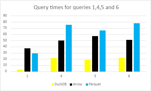
As you can see the first query is very fast. This is due to DuckDB storing metadata for each column, this includes the max, the min and if the column contains any nulls. There are two reasons for this, one is to speed up queries such as this one as max and min are extremely useful statistics, the second is about compression, consider for example the sequence 1001 1002 1003 this simply the sequence 1 2 3 shifted by 1000 numbers. Since numbers beyond certain sizes require more bytes to store this can be a way to significantly decrease the size of a column. An explanation of what is going on with compression in DuckDB can be found here, specifically the sections on Bit-packing and Reference Frame.
Queries 4,5 and 6 follow the similar trend that we had seen in our As-of join blog post, Arrow is faster than Parquet, mainly due to its in-memory capabilities and no decompression requirements, but both are slower than DuckDB native files. Query 5 slightly deviates from this trend in that Parquet and Arrow perform very similarly, but again, both fall short of the DuckDB files.
The following graph displays the times for the second query:

With no complex aggregations, just a simple filter of returning 4 rare syms, the expectation on this query is that it would be lightning quick within each filetype. The two main highlights of Query 2 is noting, firstly, that yet again the expected trend prevails, DuckDB is faster than Arrow and Arrow is faster than Parquet. Secondly, just how fast Arrow is. This is due to Arrow’s memory mapping capabilities, allowing it to find these rows efficiently. Memory mapping increases speed when accessing data on disk by storing the locations of on-disk data sections in memory, allowing us to only load the required data. For a more in depth look at memory mapping check out this blog by KX. The fact that Arrow can almost match DuckDB, especially when you consider the lack of speed compared to Parquet, is a testament to memory mapping’s capabilities.
The last graph shows the times for the third query:
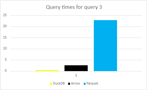
In a similar vein to query 2, the third query is simple. No aggregations, no complex and detailed filters, all that’s happening is the return of a single sym, with 600000 rows. Nonetheless, we expect the times should be quick, and we can see the times again live up to expectations. Just like query 2, DuckDB shines forth with a time of around 400 microseconds. Arrow clocks in at 2.9 milliseconds, and as usual, Parquet finishes last in the race, with a time of over 20 milliseconds.
So what? Has this in-depth analysis on the performance of 6 random queries served any purpose? Yes. On a whole, DuckDB performs well in every single category. Regardless of what you need in a query, whether it’s an incredibly selective filter, or a complex aggregate, or a bit of both, DuckDB excels. Another key takeaway from not only our current blog, but also the other blogs within the DuckDB series, is DuckDB’s ability to competently mount different filetypes, which is yet another example of the versatility and power of DuckDB. Obviously, we would be remiss to not mention the differences in the performance of the filetypes. Thus, we recommend if you want speed at the expense of not separating the data from the database, use DuckDB. If you want to keep the data and the database separate without a significant sacrifice in performance, use Arrow, and if your priority is disk space, then use Parquet.
Optimisation
As has been demonstrated throughout the series of blogs, DuckDB is very functional, and very fast. Not only that but it has a lot of features that are continually being updated and upgraded, and with the current version being 0.9.1, we thought that with all these new additions and features, we could test whether they have or can contribute to the speed of DuckDB. The main two features that we want to look at are:
- Compression
- Partitioning on sym
Compression
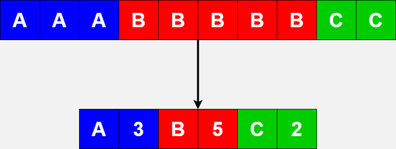
DuckDB uses a variety of compression methods, one of which is RLE (Run-length encoding). Run length encoding works as a compression algorithm in that rather than storing every element in a column, instead it will store an element and then the number of times it appears consecutively. This is particularly useful for columns with lots of consecutive repeated values such as the sym column in financial data. Since our data is sorted on time and sym, our sym column contains consecutive repeated values for each sym, and therefore, with RLE, we would essentially have a dictionary pointing to the ‘sections’ of a column that contains each sym. For example if there are 100 entries with sym A, we know that the RLE will store, A 100.
We hope that compression may be something DuckDB makes use of to speed up our queries, most importantly, queries 2 and 3, where we are searching for rare syms, and yielding a large return from just one sym. In particular if the sym column is sorted then RLE will effectively become a dictionary of exactly where to find each sym as seen below.
To test if there was any change in speed, we saved the data down uncompressed (you can choose the compression type when creating a table). The results were interesting, what we saw is that the difference for queries 2 and 3 was minimal, but looking at the compression information we saw that even if the data is stored uncompressed DuckDB still stores stats for the column segments. Thus when looking for particular syms, it can first check if it is within the range of a segment (min and max are stored) and only then does it need to actually check which rows it matches. It doesn’t seem then that the dictionary encoding within each segment provides much in terms of query speed for these kind of filtering queries.
If you want to find out more about the different compression algorithms used by DuckDB, here’s a helpful guide, as linked above.
Partition on Sym
As has been explored in a previous blog, DuckDB can support partitioned datasets. However, we wanted to take it one step further, and test if partitioning on sym would decrease the time taken for queries 2 and 3, since they are simply returning rows for specific syms. Our hope is that these filters will be pushed down into the partitions and only the required partitions will be read in and used.
| Arrow | Partitioned Arrow | Parquet | Partitioned Parquet | |
| 2 | 1.68 | 2.86 | 18 | 3.63 |
| 3 | 2.39 | 3.25 | 22.9 | 3.17 |
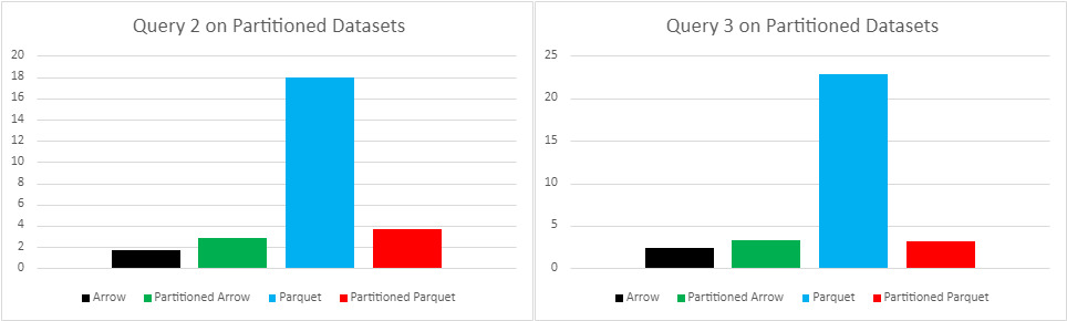
For Arrow we see that partitioning slightly slows down both of these queries, this implies that Arrow’s memory mapping is faster than the filter pushdown, proving just how efficient memory mapping is. On the other hand, for Parquet these queries both speed up drastically, this is because the filter pushdown allows us to only load the required data. So for query 2 only the ‘AIW’, ‘AUSF’, ‘BBDO’, and ‘BDR’ partitions will be loaded and for query 3 only the ‘AAPL’ partition will be loaded.
The results for query 2 and 3 on sym partitioned data clearly do provide a speed increase on parquet files; however, sym partitioning will slow down queries involving aggregations, like queries 4,5 and 6, since all partitions need to be loaded. Below is a graph that shows that the times for partitioned datasets are almost 20 times longer for each of the last three queries.
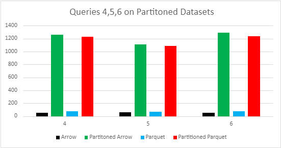
Therefore, we don’t recommend partitioning on sym in practice.
Conclusion
Unfortunately, neither of our hoped for improvements are a perfect fit for optimising these highly selective queries. This is a little disappointing but given the rate at which DuckDB has been adding features perhaps metadata is something we will see used in the near future to make these kind of queries almost instant. However the performance of all 6 queries within this study already makes DuckDB a serious competitor as a Database Management System. We definitely think it is something to keep an eye on.
Share this: