Apache Arrow, DuckDB, Polars and Vaex
Data Intellect
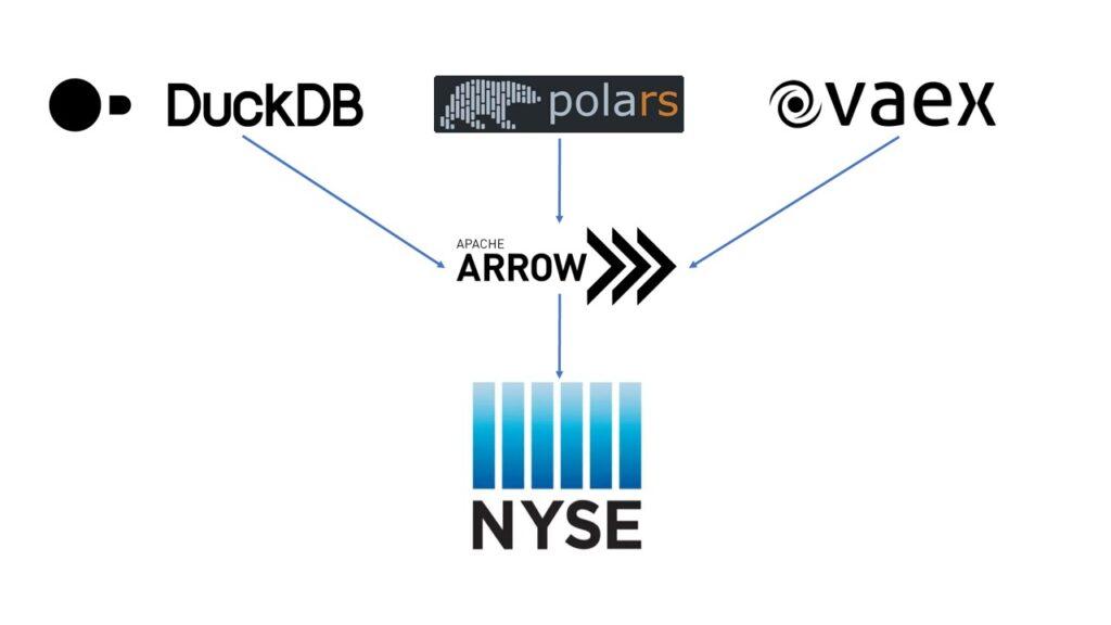
In the data science community, there are as many ways to query data as there are ways to store it. With new technologies constantly popping up, it can become overwhelming trying to decide which one is the best use for a given case. Fortunately open language-agnostic data formats, such as Apache Arrow, are gaining more and more traction. In AquaQ we deal with large tables of financial data, and in this mini-project we are going to look at three separate technologies; DuckDB, Vaex and Polars, and compare their ability to query a single day of NYSE TAQ data with the trade and quote tables stored as arrow files.
Tables are a lovely 2-dimensional grid that helps us structure and organise data. When we write tables down to memory, we have to squishify this lovely 2D grid down to a 1D sequence of zeros and ones. This leaves us a choice, do we write one row down after the other, or do we throw a whole column down to memory and then the next?
Say we have a table containing records for a company; names, ID’s, roles etc. When we consider this you can imagine why row storage makes sense. Keeping all the data related to an employee together seems sensible. How foolish…
Let’s query the data. We’re only interested in employees that think columnar storage is best. Because we’re row oriented, we skip entries until we hit the employee’s preference. We read it, then jump to the next one, read it, jump and so on. The end result is lots of little jumps that leave us with an overall feeling of getting nowhere quickly.
This outlines what makes columnar data so appealing. Don’t need a column? Do one big jump and don’t load it into RAM at all. Our datatype is the same the whole way down too; so we can run an instruction on multiple values at once. Reads are crazy fast and have constant random-access time.
Columnar storage is best for analysis which is where all the action is these days. Row storage still has its place where we’re adding new records constantly, like an online shop database. But this marks the end of her reign as champion of in memory data formats.
Arrow is an open source columnar memory standard that enjoys the benefits mentioned above. Being open source adds one more big appeal to this list – flexibility. Query your data in Python, Rust or Go without copying or converting once. No serialisation between languages or processes required; columnar databases for the masses!
Arrow Overview
First a bit on Arrow; as mentioned it is an open source memory standard and at the helm is Wes McKinney, the father of the Pandas framework. Arrow was started by Wes and others as a way to address the short comings of pandas and its numpy dependencies (10 THINGS I HATE ABOUT PANDAS). Pandas at this point is accurately described by the bear it was named after. Feeding off of bamboo it gets no nutrition, sleeping all day and when it does anything – it’ll do it when it feels like it, no rush or anything. Changing our diet to Arrow super charges the whole pipeline. Support for memory mapping, easily vectorizable operations and zero copy clones come as a side effect of switching food groups. See here for full description of what makes arrow so great.
METHOD FOR TESTING
At AquaQ financial data is our bread and butter; so to get a nice comparison going we are using a single day of the NYSE TAQ data set. This consists of a trades and quotes table with 30 and 80 million rows respectively. We have two queries to run on the smaller data set and one more to run on the larger dataset. We are going to show the query structure in each module then profile the RAM usage and speed.
Testing
Trades simple window query
Our first query is a filter window which selects the opening trade for Apple. For more details check out the repo on GitHub.
DuckDB
con.query("SELECT * FROM trade WHERE Symbol = 'AAPL' AND Sale_Condition LIKE '%O%'").df()DuckDB uses SQL to query the data. The simplicity and familairity of SQL makes using DuckDB a breeze if you’re familiar with QSQL like we are here at AquaQ. As DuckDB is embedded, queried data can be sent between different DataFrames with zero copying (no extra memory) by adding the desired format at the end of the query; .fetchall() for the native format, .df() for a pandas DataFrame, .pl() for a polars DataFrame, and more.
| Time | Exchange | Symbol | Sale_Condition | Trade_Volume | Trade_Price | … | Participant_Timestamp | |
|---|---|---|---|---|---|---|---|---|
| 0 | 2019-10-07 09:30:00.562307 | Q | AAPL | @O X | 223839 | 226.26 | … | 2019-10-07 09:30:00.562284 |
Polars
trade.filter(
    (pl.col("Symbol") == "AAPL")&
    (pl.col("Sale_Condition").str.contains("O"))&
    (pl.col("Time").is_between(datetime(2019,10,7,9,30), datetime(2019,10,7,16,0)))
).collect()
Polars takes after pandas in its DataFrame framework. With a similar syntax using filter statements we can achieve the same effect as a where clause in SQL.
Vaex
trade[(trade['Symbol'] == 'AAPL') &
    (trade['Sale_Condition'].str.contains('O')) &
    (trade['Time'] >= np.datetime64('2019-10-07 09:30')) &
    (trade['Time'] <= np.datetime64('2019-10-07 16:00'))]
Vaex is very similar to polars in syntax with slightly less clear but shorter notation using square brackets instead of the filter keyword.
—–
DuckDB is clearly the most concise of the three options and also performs the best. The expressions of polars and vaex is familiar for anyone familiar with pandas. Polars had some problems with this query, we narrowed this down to the dataset scanner method which is experimental in implementation, which when removed resulted in a massive reduction in memory.
Trades aggregate
Getting a bit more complex now; we are going to sum the volume by symbol and hour time bucket across the day.
DuckDB
con.query("SELECT DATE_TRUNC('hour',Time) AS hour, SUM(Trade_Volume), Symbol FROM trade GROUP BY hour, Symbol ORDER BY hour").df()Initially DuckDB had trouble with time bucketing the data, as the new development version‘s time_bucket function was producing segmentation fault errors (something that may be shortly patched). However after some teething issues adapting to SQL query syntax, the date_trunc function was still able to truncate the data successfully and produce the desired table.
| hour | sum(“Trade_Volume”) | Symbol | |
|---|---|---|---|
| 0 | 2019-10-07 04:00:00 | 101.0 | CEI |
| 1 | 2019-10-07 04:00:00 | 45.0 | PCG |
| 2 | 2019-10-07 04:00:00 | 3.0 | CNC |
| 3 | 2019-10-07 04:00:00 | 135.0 | TEN |
| 4 | 2019-10-07 04:00:00 | 55.0 | OHI |
| … | … | … | … |
| 75015 | 2019-10-07 20:00:00 | 100.0 | INDS |
| 75016 | 2019-10-07 20:00:00 | 100.0 | RETL |
| 75017 | 2019-10-07 20:00:00 | 17823.0 | XXII |
| 75018 | 2019-10-07 20:00:00 | 100.0 | YCS |
| 75019 | 2019-10-07 20:00:00 | 4954.0 | SVM |
Polars
# sort the data first
trade = trade.sort("Time")

# query
trade.groupby_dynamic(index_column="Time", every="1h", period="1h", by="Symbol").agg(
[
    pl.col("Trade_Volume").sum().alias("Total_vol")
]).collect()
Polars has a nice time bucket method built in, easy to use and reliable. Too good to be true? Indeed, the data MUST be sorted on time, even though data is continuously sorted on time by sym there is no way to tell polars (that I found) that its already sorted. Good thing polars sorts are optimised or we would be in trouble.
Vaex
trade.groupby(by = [trade.Symbol,vaex.BinnerTime(quote.Time,'h')],
    agg = {"Total_vol": vaex.agg.sum("Trade_Volume")})
Vaex again has similar syntax to Polars with its own nice time binning method. This was a nightmare, finding documentation was impossible and binning on one minute would break the whole method. We changed the whole test to bin on hours so we could compare vaex. My experience here was frustrating leaning towards enraging.
Quotes aggregate
On the bigger dataset we are calculating the average mid price for each symbol and hour time bucket.
DuckDB
con.query("SELECT DATE_TRUNC('hour', Time) AS hour, Symbol, AVG(0.5*(Offer_Price+Bid_Price)) AS mid FROM quote GROUP BY Symbol, hour ORDER BY hour").df()Like the previous queries, DuckDB had no struggle with this aggregation over the huge quote table. The time bucketin was again done with the date_trunc function, and the syntax of the query is clear if you know SQL.
| hour | Symbol | mid | |
|---|---|---|---|
| 0 | 2019-10-07 03:00:00 | SOL | 0.000000 |
| 1 | 2019-10-07 04:00:00 | SSW | 4.805000 |
| 2 | 2019-10-07 04:00:00 | SCPE U | 5.105000 |
| 3 | 2019-10-07 04:00:00 | STKL | 3.445000 |
| 4 | 2019-10-07 04:00:00 | SOHO B | 22.842500 |
| … | … | … | … |
| 9190 | 2019-10-07 20:00:00 | SVT | 1.583333 |
| 9191 | 2019-10-07 20:00:00 | SZC | 4.997500 |
| 9192 | 2019-10-07 20:00:00 | SD | 1.795000 |
| 9193 | 2019-10-07 20:00:00 | SPE PRB | 0.000000 |
| 9194 | 2019-10-07 20:00:00 | SPXL | 40.594048 |
Polars
# sort the data first
quote = quote.sort("Time")

# query
quote.groupby_dynamic(index_column="Time", every="1h", period="1h", by="Symbol").agg(
[
    (0.5*(pl.col("Bid_Price")+pl.col("Offer_Price")).mean()).alias("mid"),
        pl.col("Time").min().alias("min_time"),
        pl.col("Time").max().alias("max_time")
]).sort("Time").collect()
Pretty much a repeat of above, bucketing works lovely if you sort on time and the syntax is lovely and clear. No issues here, we’ll discuss memory and performance at the end however…
Vaex
quote.groupby(by = [quote.Symbol,vaex.BinnerTime(quote.Time,'h')],
    agg = {'mid': vaex.agg.mean('Offer_Price+Bid_Price/2')})
Vaex continues to work nicely, binning on one minute works fine on this dataset, even though the type and format is identical. Weird… I’m missing something but part of this writeup is useability and Vaex time binning is not user friendly.
Memory and Performance
The arrow files for the trade and quote tables are 3.4GB and 13GB respecively. We profiled the peak memory utilisation and CPU wall time for each query on each framework. Below are the results in a chart format for your comparison pleasure, showing the memory usage for each query for each technology respectively measured in gigabytes (GiB). It would be good to reiterate that we are by no means experts in any of these modules. There are no doubt better ways to query than we have.
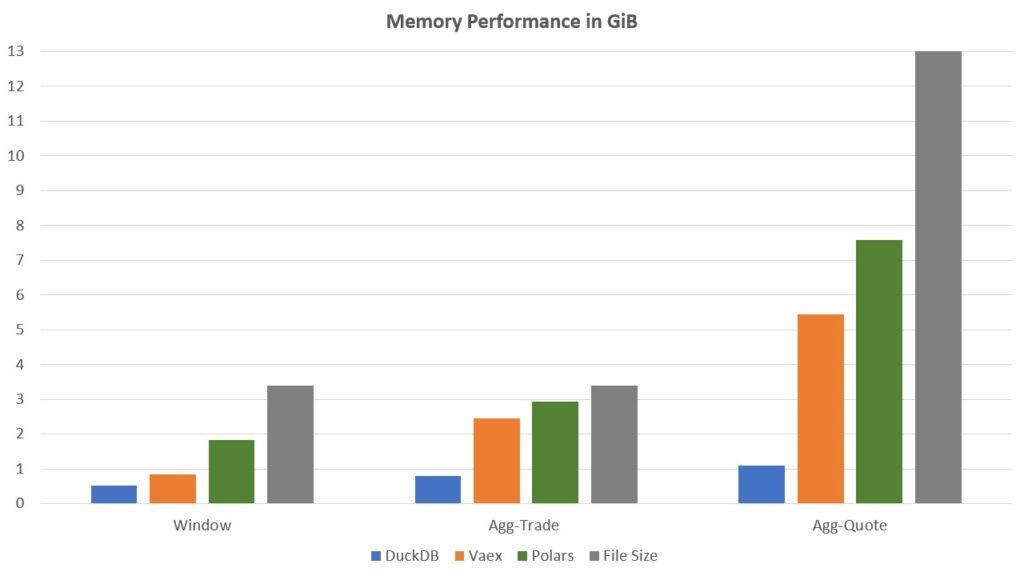
DuckDB mops the floor with everything here, consistently using the least memory while also having the shortest query time. The developers have done a great job. Polars is very disappointing, though it should be noted that in their own benchmarks they excel in joins which was not explored here. Vaex sits between the two being just alright.
Conclusion
Performance wise DuckDB steals the show, its really impressive what their team have managed to create. It’s SQL based query framework is very appealing as the language is widely used and comes with a lot of documentation. On the other hand those more familiar with pandas in the data science community may find comfort in the pandas-like expression structure that polars and vaex bring to the table. Polars in particular has some very powerful expression methods built in that can modify values based on conditions elsewhere in the table.
But why pick a favourite? They all have their strengths, and with arrow as the backbone we can pass data between each module with no copying or serialisation. Filter with DuckDB and use 1GB of memory on 80 million rows. Then pass to Polars to modify based on a condition. The flexibilty provided by arrow is the real star of the show here.
The space moves so fast it’s hard to keep up. The long awaited pandas 2 electric boogallo is set to release this month. With its beautiful new pyarrow backend it will be worth a look at to see how it stacks up against the competition. Pyarrow itself is due to release version 12 as well, maturing its new dataset methods. This looks like the springboard that columnar storage needs. The future looks fast.
Share this:


