Apache Arrow and Partitioned Datasets
Aaron Capper
Authored By: Carla McLaverty and Aaron Capper
Apache Arrow is an open-source software project that provides a columnar in-memory data format. This is a similar software/file type to Apache Parquet, but Parquet is instead optimised for disk-based storage.
This blog post is a follow on from a previous Data Intellect post which investigated the various means of querying data stored in arrow format. Throughout the course of that project, we found DuckDB easy to use with its intuitive SQL based query framework and found that it consistently resulted in lower query times and memory usage, when compared to similar software packages. This is due to DuckDB’s ability to push filters and projections directly into arrow file scans and then only read the relevant columns and partitions into memory.
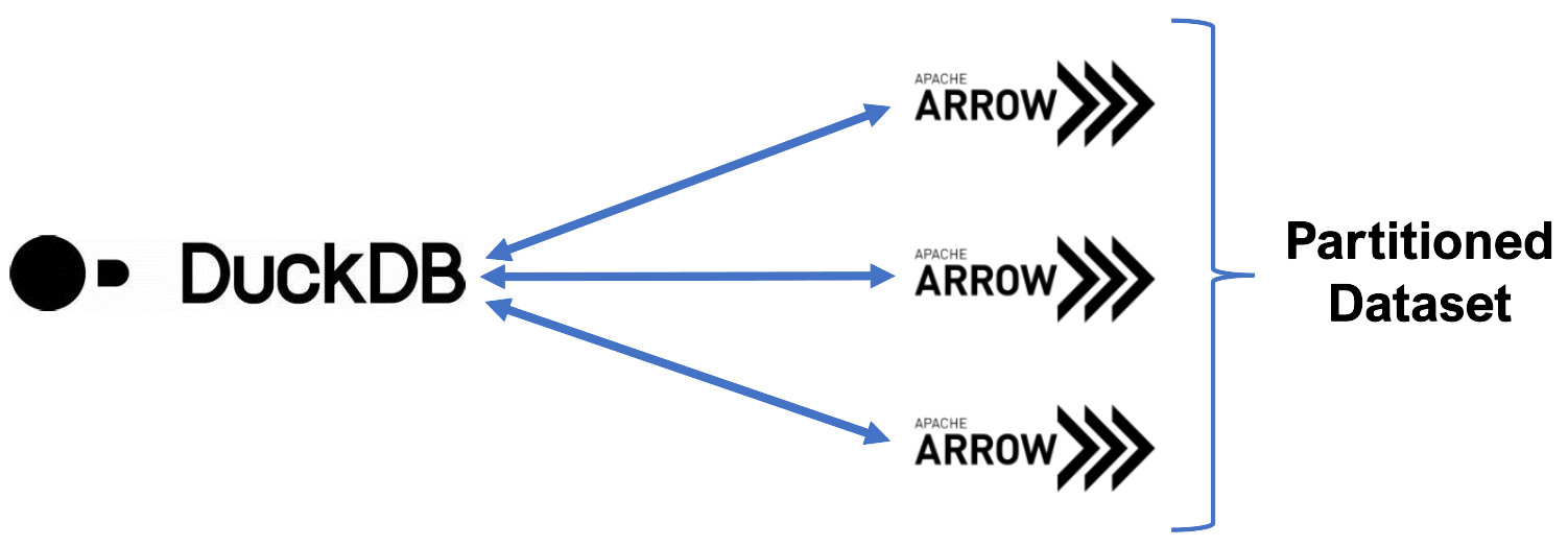
Since the completion of the aforementioned project Arrow has released a new feature, pyarrow.dataset, which makes it easier to query tabular datasets that can potentially be larger than memory, and partitioned datasets. This new feature makes filtering and projecting columns within partitioned datasets easier. Partitioned datasets are useful in today’s data driven world as they handle large volumes of data especially well. They handle time series data particularly well as that data has a natural partitioning key of time periods (e.g. dates). They are easily scalable while keeping the data organised logically. Like columnar formats, partitioning can improve query performance by limiting the amount of data that must be scanned or processed.
Here at Data Intellect, we are very familiar with partitioned datasets as they are extensively used within the finance industry (one which we work within frequently), and so we decided to investigate the effectiveness of querying partitioned datasets in the new arrow file format. We tested this by running some routine queries and inspecting their results by means of memory and timing measurements. Within financial data, trade and quote tables are common and so we created a database with one of each table within each partition. For further query analysis we decided to focus on the trade table, as it is more recognisable and easily understood by those who are unfamiliar with these types of tables.
.
└── month=04
    ├── day=21
    │   ├── quote
    │   │   └── part-0.arrow
    │   └── trade
    │       └── part-0.arrow
    └── day=22
        ├── quote
        │   └── part-0.arrow
        └── trade
            └── part-0.arrow
This snapshot shows an example of a small database formatted as described above.
Whilst loading in the partitioned database it is possible to use a predefined partitioning schema within the pyarrow.dataset.partitioning function, such as the “hive” schema which partitions directories as key value pairs. However, we found this schema to be awkward and inefficient to query, as to query a date you had to specify the year, month and date of the required data (as shown by the directory structure above). While this was manageable when querying a single date, it proved to be bothersome while trying to query date ranges etc. Instead, we defined our own partitioning schema, that is shown below, which created a virtual date column across the tables. This date column was cast to type64, which then allowed us to pass singular dates as well as date ranges much more intuitively through our queries.
part = pyarrow.dataset.partitioning ( pa.schema([("date", pa.date64())]) ) We began by creating a database with 100 partitions to query. Each of these partitions consisted of one day’s worth of mock trade and quote data with 100,000 and 500,000 rows respectively. These tables were then saved down as csvs in their partitioned structure, before being converted to arrow files using pyarrow. The resulting database equated to 2.86 GB on disk. The size of this database was much less than the memory available on the system (approximately 40-60GB RAM free out of a total 125GB at any given time), and so posed no threat of overloading the system when queried. However, we found that we were only able to define one table schema per session, and so we separated the trades and quotes tables into different directory structures (sizing 361Mb and 2.5GB respectively). These databases could then be mounted and loaded in separately with each table retaining its correct schema.
.
├── arrowquote
│   ├── 2014-04-21
│   │   └── part-0.arrow
│   └── 2014-04-22
│       └── part-0.arrow
└── arrowtrade
    ├── 2014-04-21
    │   └── part-0.arrow
    └── 2014-04-22
         └── part-0.arrow
This snapshot shows the directory structure following separating the tables and creating the arrow files with the custom partitioning schema, for each day of mock data. This snapshot shows just 2 out of the total 100 partitions as a means of demonstration, however all the other partitions follow the same format.
We began by querying “select * from trade”, as shown below, and analysed its memory and timing stats using %memit and %timeit. This initial query was then used as a benchmark for the results of our following queries, as this query loads into memory all the mock trade data from our database.
con.query("SELECT * FROM trade").df()
> peak memory: 4479.57 MiB, increment: 3869.37 MiB
> 3.59 s ± 220 ms per loop (mean ± std. dev. of 7 runs, 1 loop each)| sym | time | src | price | size | date | |
|---|---|---|---|---|---|---|
| 0 | AAPL | 2014-04-21 08:00:01.730 | O | 25.40 | 1958 | 2014-04-21 |
| 1 | AAPL | 2014-04-21 08:00:05.606 | L | 25.37 | 3709 | 2014-04-21 |
| 2 | AAPL | 2014-04-21 08:00:12.838 | N | 25.34 | 1684 | 2014-04-21 |
| … | … | … | … | … | … | … |
| 10245972 | YHOO | 2014-09-05 16:29:50.558 | O | 16.49 | 4199 | 2014-09-05 |
| 10245973 | YHOO | 2014-09-05 16:29:51.541 | N | 16.52 | 834 | 2014-09-05 |
| 10245974 | YHOO | 2014-09-05 16:29:56.387 | L | 16.49 | 1051 | 2014-09-05 |
10245975 rows × 6 columns
Before running each of the following queries, we made sure to restart the kernel. This ensured that our memory statistics wouldn’t be impacted by the potential of having the data preloaded into cache from the previous query. This allowed us an accurate representation of how much data is needed to be pulled into memory each time the query is run, regardless of what was queried prior.
We took into consideration the peak memory used, and more specifically the memory increment of each query when analysing our results. The peak memory measurement refers to the largest amount of memory used by the system during the query runtime. This would include any memory cached before our query is ran as well as the memory used to run our query, but gives us an idea of the maximum amount of memory required to be available at the time of running the query, for it to execute successfully. The memory increment measurement is the equivalent of the peak memory minus the starting memory value (i.e. the memory in use by the system immediately before running the query). As such, this value gives us a better idea of how much memory the query itself takes to run.
con.query("SELECT * FROM trade WHERE date=='2014-04-25'").df()
> peak memory: 633.81 MiB, increment: 23.53 MiB
> 38.7 ms ± 4.18 ms per loop (mean ± std. dev. of 7 runs, 10 loops each)We can see that the amount of memory required for this query dropped significantly in comparison to our initial select * from trade query. This query is asking for just one trades partition to be returned instead of the whole database, and the drop in memory needed here shows that the system is indeed responding to this query and allowing DuckDB to only load in the required sub-selection of data, as a result.
con.query("SELECT date,sym,MAX(price) FROM trade WHERE date BETWEEN '2014-06-02' AND '2014-07-31' GROUP BY date, sym ORDER BY sym,date").df()
> peak memory: 707.39 MiB, increment: 97.44 MiB
> 44.9 ms ± 1.05 ms per loop (mean ± std. dev. of 7 runs, 10 loops each)| date | sym | max(price) | |
|---|---|---|---|
| 0 | 2014-06-02 | AAPL | 17.19 |
| 1 | 2014-06-03 | AAPL | 16.53 |
| 2 | 2014-06-04 | AAPL | 17.23 |
| … | … | … | … |
| 393 | 2014-07-29 | YHOO | 17.29 |
| 394 | 2014-07-30 | YHOO | 17.35 |
| 395 | 2014-07-31 | YHOO | 16.82 |
396 rows × 3 columns
This query is more complex than the previous; it applies an aggregator, selects from within a date range and asks for the data to be ordered as specified (the result of this query is the table shown above). These resulting memory statistics are slightly higher than the previous query, yet still significantly lower than the initial select * from trades. This is impressive considering the complexity of the query, and the fact that it is required to crawl through 2 months of data to produce these results. This once again shows DuckDB’s capability to limit the data loaded into memory to only that which is required.
The time taken to complete each query follows a similar trend to that of memory. Whilst the speediness of a query is important to consider, especially for financial markets where time quite literally equals money, this is a slightly less reliable means of comparison than memory. The time taken for the query can vary anywhere from slightly to drastically depending on what other operations are taking place on the server at the same time. However, the trend shown in these results is consistent with what we expected, as less memory is loaded and searched, the time taken for the query similarly reduces.
For the next example, we created a 100GB database. This database is larger than memory and if loaded into memory, would crash our server, but it was created to demonstrate pyarrow’s capabilities for mapping such large datasets along with DuckDB’s ability to push filters and projections into arrow scans (even as far as datasets bigger than memory). We ran a simple select query across a range of filters, in order to pull one specific row from the large database.
con.query("SELECT price,size FROM trade WHERE date == '2014-04-23' AND sym=='AAPL' AND time=='2014-04-23 11:06:40.059'").df()
> peak memory: 248.19 MiB, increment: 80.57 MiB
> 337 ms ± 5.08 ms per loop (mean ± std. dev. of 7 runs, 1 loop each| price | size | |
|---|---|---|
| 0 | 25.45 | 37 |
As can be seen, this is not only possible but also highly memory and time efficient. The memory required to execute this query is vastly smaller than if we had have pulled the whole database into memory. This further proves, on a larger and more obvious scale, that pyarrow only maps the database to memory and that DuckDB pulls only the selected columns into queries, saving us from a potential server crash…
CONCLUSION
During our investigation we showed that Pyarrow’s new version 12 will allow you to combine the speed and efficiency of loading tables stored using arrow files, with their on disk columnar based storage, and the convenience of using a partitioned database. Pairing this new software with the ease of querying using SQL with DuckDB, made querying partitioned datasets a breeze.
Alongside this, it is very common to find large volumes of real market data stored as a date partitioned database within the financial sector; therefore, we can conclude this project to be a success as it demonstrates a real-life application using Pyarrow and DuckDB.
Although we did use DuckDB for this investigation, it is possible to use many other softwares to query arrow files. Our previous blog post gives an overview of some of these other options.
It was also seen that not only could Pyarrow and DuckDB be used to successfully load in a partitioned dataset, but they could also load in a dataset larger than memory. This successfully shows that the pyarrow.dataset.dataset function doesn’t actually read the data into memory, it just crawls the directories to find the files and maps these to memory. Pyarrow also successfully created a virtual date column when loading in the partitioned dataset based off the partitioning schema, which allows users to query tables by date even when no date column is present in the tables. DuckDB’s optimized filtering and projection was then used to load only the queried data into memory.
During our investigation we used Pyarrow and DuckDB to load and then query the partitioned datasets, however it is possible to query and load the partitioned datasets using Pyarrow alone. If the investigation was to be extended, this could be an interesting possibility to further explore.
Share this: