Joel Davison

Authored by Joel Davison and Jamie Peters

DuckDB has featured in two previous blog posts at Data Intellect. The first of these compared queries on an Apache Arrow dataset using DuckDB, Polars, and VAEX, and our most recent post in this series which looked at partitioned datasets in Apache Arrow. Given the results of these blogs and DuckDB’s easy-to-use SQL-based queries, we decided to explore further some of the new features DuckDB has to offer, this blog focuses on the DuckDB as-of, and there will be more to come.

As-of joins are not something you would encounter in most databases, because they don’t operate on ordered data. When dealing with unordered data one can use a variety of joins such as inner, left, and outer joins, however, if we attempt to use these on time-series data it will not work as we hope, since it is unlikely there are exact matches on the time column we will get no return or null columns. This is where the as-of comes in, it is a join that can be used on ordered data to find the nearest event in a reference table. At Data Intellect, we deal heavily with a type of ordered time series data, in particular, large financial tables of trade and quote data, and therefore the as-of join is of great interest to us.

Let us first introduce our trade and quote data and then we will demonstrate how the as-of works. Our trade and quote tables have 5 million and 15 million rows respectively, and here are the first 5 rows of each:

	sym	time	src	price	size	date
0	AAPL	2014-04-21 08:00:00.221	L	25.37	92	2014-04-21
1	AAPL	2014-04-21 08:00:01.470	N	25.27	6963	2014-04-21
2	AAPL	2014-04-21 08:00:01.927	O	25.28	249	2014-04-21
3	AAPL	2014-04-21 08:00:02.483	L	25.27	2026	2014-04-21
4	AAPL	2014-04-21 08:00:02.718	L	25.31	5174	2014-04-21

	sym	time	src	bid	ask	bsize	asize	date
0	AAPL	2014-04-21 08:00:00.075	O	25.34	25.36	9000	7500	2014-04-21
1	AAPL	2014-04-21 08:00:00.161	L	25.34	25.37	4000	7500	2014-04-21
2	AAPL	2014-04-21 08:00:00.280	N	25.33	25.36	7500	10000	2014-04-21
3	AAPL	2014-04-21 08:00:00.815	L	25.32	25.35	7000	8000	2014-04-21
4	AAPL	2014-04-21 08:00:00.880	N	25.30	25.31	9000	8000	2014-04-21

As you can see, the times for trades and quotes do not align but we want to know what the specific quote data was when the trade occurred, but as mentioned above, if we try to use any of the rudimentary SQL joins found in most databases, we run into problems. As-of joins differ from the others because an as-of join joins based on the most recent match of a specified column. In other words, the tables are joined by selecting the row with the closest column value less than the value in the row we are joining to.

Within DuckDB, there is more than one way to carry out the as-of join:

con.query("SELECT * FROM trade t ASOF JOIN quote q ON t.time >= q.time AND t.sym=q.sym AND t.src=q.src AND t.date=q.date")
con.query("SELECT * FROM trade t ASOF JOIN quote q USING (sym, src, date, time)")

The syntax for the as-of can seem quite confusing at first glance, however, when broken down it’s fairly intuitive. We first have the SELECT clause followed by the columns we want to select (or * for all) followed by our tables separated by the ASOF JOIN statement. Finally we can choose either an ON or USING clause, both clauses include the same elements – the columns to match and that will be joined on. They differ in how the columns are included in the clause. For the ON clause, each column must be given as either an inequality or an equality. Where the columns are equal (date, sym, src in our example), use an equals sign. However, the column that the ‘as-of’ functionality applies to requires an inequality. In our example, we used trade time >= quote time because we wanted the most recent quote data for a given trade. Note that the order of these tables is important, it is the second table that will be joined to the first.

The USING clause is simpler; all that is required is a list of the columns you want to match on, with the column listed last being joined with an inequality, while the other columns require exact matches. Due to its simpler syntax and faster join, we opted for the using clause.

Here is a snapshot of the table produced by the as-of join, returning the sym, time, price, bid, ask and quote time columns from the trade and quote tables:

	sym	src	time	price	bid	ask	quote_time
0	AAPL	L	2014-04-21 08:00:00.221	25.37	25.34	25.37	2014-04-21 08:00:00.161
1	AAPL	L	2014-04-21 08:00:02.483	25.27	25.27	25.31	2014-04-21 08:00:02.416
2	AAPL	L	2014-04-21 08:00:02.718	25.31	25.26	25.31	2014-04-21 08:00:02.569
3	AAPL	L	2014-04-21 08:00:03.855	25.29	25.26	25.29	2014-04-21 08:00:03.622
4	AAPL	L	2014-04-21 08:00:04.036	25.26	25.23	25.26	2014-04-21 08:00:04.000
…	…	…	…	…	…	…	…
4914038	YHOO	O	2014-04-25 16:29:57.687	62.08	62.08	62.13	2014-04-25 16:29:57.673
4914039	YHOO	O	2014-04-25 16:29:58.435	62.17	62.17	62.18	2014-04-25 16:29:58.381
4914040	YHOO	O	2014-04-25 16:29:59.914	62.09	62.09	62.14	2014-04-25 16:29:59.878
4914041	YHOO	O	2014-04-25 16:29:59.959	62.14	62.09	62.14	2014-04-25 16:29:59.878
4914042	YHOO	O	2014-04-25 16:29:59.997	62.10	62.09	62.10	2014-04-25 16:29:59.991

4914043 rows × 7 columns

The last column shows that it is the data from the last quote before each trade that is joined.

STORING THE DATA

Now that we know that the as-of works, and how it does so, we compare performance for data stored in three different files types. This is another helpful feature of DuckDB: the ability to mount different file types. As we’ve noted in our previous blogs, DuckDB can handle Apache Arrow files. However, it doesn’t stop there, DuckDB is capable of managing multiple different file types. We opt to look at three which all store the data in a columnar format:

Apache Arrow: for flat and hierarchical data, and is organised for efficient analytic operations, it focuses on in-memory data processing and presentation
Apache Parquet: provides efficient data compression and encoding schemes with enhanced performance to handle data in bulk, focuses on efficient columnar storage on disk
DuckDB: focuses on efficient query handling and data retrieval

The particularities of each file type is exemplified by the space that they occupy, our 5 million rows of trade, and 15 million rows of quote data, occupy approximately 1GB for both Arrow and DuckDB, with Parquet occupying roughly 250MB.

IT'S ABOUT TIME

Another aspect of the as-of that we want to investigate is speed, we explore this using the inbuilt python function, %timeit. This function carries out the command 7 times, then gives the mean time as well as the standard deviation.

DUCKDB’S MAGIC

When we first timed the joins, it had the illusion of performing unimaginably fast, 60 nanoseconds to be precise. However, we soon discovered that DuckDB has some tricks. Specifically, when queried, DuckDB retrieves only the data that will be displayed the console. This is useful because it quickly provides an output and a snapshot for the user. Although, when it comes to timing this creates a unique problem. We could not find an inbuilt function to time the full join, the solution we used was to materialise all the data.

We achieved this by converting every query output to a pandas dataframe using .df(). Forcing the data to be materialised allows for a more accurate reading of the performance. Other alternatives to .df() that can be used are .pl() for polars, and .fetchall() for DuckDB formatting, for aesthetic reasons, we choose .df(). It’s important to note that converting data format will not dominate query time.

Time for Results

We used the same trade and quote data for each storage format, with entries of roughly 5 million and 15 million respectively. Using the %timeit function on the same query as above, we will see the performance of each of the three formats:

From the above table, the fastest as-of join across the three formats is when the data is stored sorted within the DuckDB native format, with arrow taking marginally less time than its Apache counterpart. While it isn’t expressly clear why DuckDB’s performance is superior, there are a number of potential reasons. Firstly, the structures used to store DuckDB files are designed for efficient query handling and Apache Arrow’s primary focus is in-memory data representation, with Parquet’s focus being efficient storage. So there isn’t the same focus on efficiency and optimisation of queries in Apache Arrow. Another reason for the superior performance of DuckDB files is the utilising of join algorithms, whereas Apache Arrow and Parquet don’t seem to have such algorithms.

As would be expected, when querying for selected columns, rather than all columns, the time decreases.

	DataFormat	SortedTime_s	UnsortedTime_s
0	Arrow	8.75 ± 104ms	14.5 ± 164ms
1	Parquet	8.95 ± 231ms	14.7 ± 172ms
2	DuckDB	6.72 ± 245ms	22.3 ± 546ms

It is clear that when the data is unsorted, the times increase, with the arrow and parquet files increasing by just less than a factor of 2 and the DuckDB increasing by around a factor of 3. This change isn’t to do with DuckDB tracking that the data is sorted with indexes as you may have come across in similar contexts, but rather a direct result of better memory access patterns.

DuckDB doesn’t make any assumptions about the data, and so it sorts the data regardless before performing the as-of join. This sorting is the reason the join on unsorted data performs worse. A reasonable question to ask is, why sort if it decreases performance? Having the data sorted is paramount to having the duration of the as-of be manageable. As discussed the as-of join finds the nearest quote before a given trade, then when moving on to the next trade (which occurs after since the data is sorted) it can begin the search from this quote since the prevailing quote for the next trade must come after the original quote. So at every step, a smaller and smaller dataset is being searched, rather than scanning the data for every single trade data point. Sorted lists can be scanned using a binary search, which is a lot quicker, (O(log n) vs O(n)) and this may be utilised by DuckDB. To put it into perspective, it takes much less than a second for DuckDB to pull in 10 million rows. The fact that the joins are taking almost 10 seconds is most likely due to the sort. Therefore, on the sorted data, sorting adds time that could be avoided if assumptions were made about the data or the data was checked for sortedness.

However, while DuckDB doesn’t carry out any checks on the data right now, this could change in the future. They plan on introducing changes to the as-of that tracks the metadata of tables, meaning that if the data is sorted, the sorting step will be skipped, and the as-of’s time will be even quicker as the dominant factor will not be carried out. Improvements like these have happened already at DuckDB, they have already reworked the as-of once and made big performance gains. For more upcoming changes within DuckDB, check out their GitHub.

In regards to the DuckDB files being the slowest on the unsorted data, it seems to be down to the fact that the Arrow and Parquet files are partitioned, whereas the DuckDB files are not. When the Arrow and Parquet files are loaded without a partitioning schema, the time for the as-of increases to a similar time to the DuckDB files. The unsorted data used in this investigation is unsorted within each partition, and so the sorting algorithms will still be gaining from this partial ordering.

Slippin' and Slidin': The as-of in practice

It’s all well and good looking at how fast as-of joins are, “But when are they useful?” I hear you ask. Our example is transaction cost analysis (TCA), which involves looking at execution costs, and whether they match expected costs. Specifically, we are looking at slippage which is the difference between the expected price of a trade and the executed price. It is fairly intuitive how as-of joins apply to TCA, one can compare data of the execution of a trade, including the executed price with the most recent bid, and ask from a quote table.

If we use our trade table, and make some mock execution data, then we can as-of join the execution data to the prevailing quote, and analysis can be carried out. Onto this new table we add a mid price for each trade, which is the average of the bid and ask, and take that as an estimate for the market price of the trade.

	sym	time	src	price	bid	ask	mid
0	MSFT	2014-04-21 08:02:26.436	N	36.36	36.36	36.38	36.370
1	AAPL	2014-04-21 08:12:19.418	N	25.83	25.83	25.87	25.850
2	ORCL	2014-04-21 08:32:39.438	L	31.91	31.91	31.93	31.920
3	DELL	2014-04-21 08:34:08.893	L	28.64	28.61	28.63	28.620
4	MSFT	2014-04-21 08:36:17.769	N	38.84	38.79	38.80	38.795
…	…	…	…	…	…	…	…
420	MSFT	2014-04-25 16:12:15.130	O	52.78	52.74	52.77	52.755
421	MSFT	2014-04-25 16:13:21.115	O	53.09	53.10	53.16	53.130
422	MSFT	2014-04-25 16:16:44.303	O	53.49	53.50	53.53	53.515
423	MSFT	2014-04-25 16:23:53.031	N	55.22	55.22	55.23	55.225
424	MSFT	2014-04-25 16:24:30.334	O	55.23	55.20	55.22	55.210

425 rows × 7 columns

From this table, we can create a histogram showing the volume of trades executed and the price they were executed at relative to the mid, in terms of half-spread:

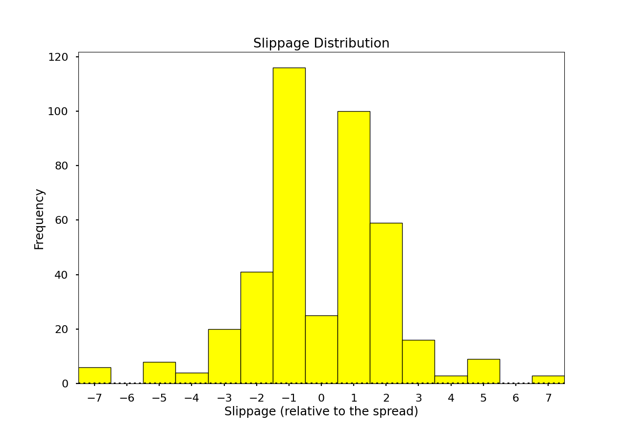
We can see most trades are executed at the bid and ask (1 and -1), but we have some outliers, these trades executed away from the bid/ask could be because of a variety of reasons. Low liquidity or a high order size could lead to the best bid/ask being exhausted and some of the trades being executed at a worse price. Alternative factors such as overnight/weekend gaps in trading, high latency, and volatility could lead to trades further from the ask/bid in either direction.

Overall there are a variety of reasons why such trades might be occurring. In practice one would need to analyse these further, looking for trends causing this slippage and constructing a plan to avoid them if they are detrimental. For this blog, we feel it is sufficient to demonstrate that this kind of analysis is possible with DuckDB and in particular the as-of join.

Disclaimer: We are using mock data, this is for demonstration purposes only and may not perfectly reflect real-life data

If you are interested in finding out more about DuckDB’s as-of joins, have a look at this post from the DuckDB blog.