Performing Beta Analysis on Stocks, Indices and Commodities Futures

Introduction

Often an investor will want to determine whether a stock moves in the same direction as the rest of the market, a portfolio, or some combination in between. There are a few reasons why an investor would want to do this but a common one is to gauge how much risk a new stock is adding to a portfolio.

A common technique to help answer these questions is Beta analysis.

This post shows how to use a simple linear regression using ordinary least squares to calculate the Betas of the returns of a simple basket of securities compared to an underlying stock.

It assumes a simple working knowledge of the following python data science and simple statistic topics, specifically

DataFrames, Filters, Joins, Sorting, Collections and Comprehensions, User Defined Functions, Python Resource Managers, Regression Analysis, Dependent and Independent Variables

Supporting material containing csv files and notebooks for this post can be found in the Beta Analysis folder in this Repo.

 

 

It contains 2 notebooks

• One that uses the yfinance package to download market data from yahoo finance
• One that performs the regression analysis

The scenario

An investor has access to a basket of the following securities

• The SP500 (assume a passive ETF tracking this index)
• Futures in Oil, Gas and Gold

They want to know how the daily returns on Halliburton, an American corporation specialising oil field service, moves compared to the constituents of this basket with a confidence level of 95% or greater in their findings.

The technique used here is

1. take daily closing prices for each security in question
2. calculate the daily return for each security
3. perform an ordinary least squared regression to calculate the coefficients (betas) for the independent variables (the basket constituents)

This is a surprisingly easy problem to solve using the pandas and statsmodels packages and some elementary data science functions.

Regression Analysis

Step 1 — Import the appropriate python packages

import pandas as pd
import numpy as np
import matplotlib.pyplot as plt
import seaborn as sns

Step 2 — Import market data

Import the dependent and independent variables. For convenience these are stored in 2 separate csv files

df_HAL = pd.read_csv(filepath_or_buffer='../Data/HAL.csv', 
                     parse_dates=True, 
                     index_col='Date')

df_basket = pd.read_csv(filepath_or_buffer='../Data/basket.csv',
                        parse_dates=True,
                        index_col='Date')
 

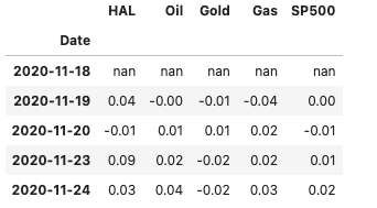
Concatenate both datasets and display the first 5 rows

df = pd.concat(objs = [df_HAL, df_basket], axis = 1)

df.head()

Most of the time analysts are more interested in the daily returns of securities and not their actual daily prices. There are a few ways to calculate these, here I am using the convenience method pct_change()

df = df.pct_change()

df.head()

Step 3 — Perform the regression analysis

This step uses the statsmodels package to perform an ols regression to solve the following model

The statsmodels function to solve the above equation is

import statsmodels.formula.api as smf

model = smf.ols(formula="HAL ~ SP500 + Oil + Gold + Gas", data=df)

And to fit the model

result = model.fit()

result.summary()

Step 4— Interpret the results

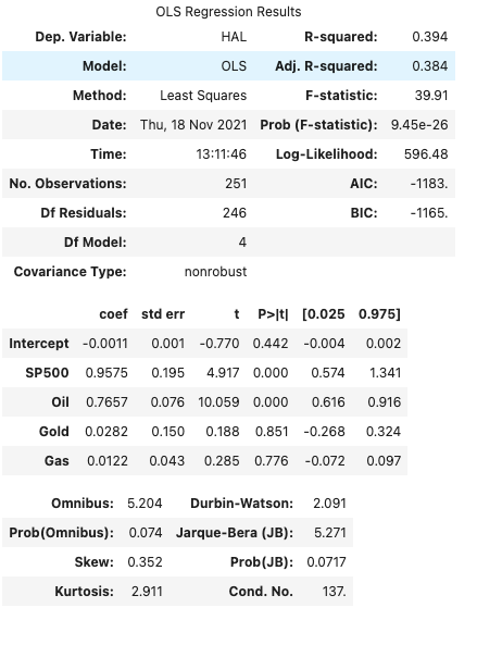
The top of the model displays a summary of the regression, the dependent variable, model, method, number of observations etc.

R-squared — how much the dependent variable is explained by changes in the independent variable(s). For this example, the model explains 39.4% of changes in the HAL variable.

The middle table shows the coefficients (Betas) for each independent variable and their corresponding p-value

Coef — the beta for each independent variable

P > |t| — uses the t statistic to produce the p value, a measure of how likely the coefficient happened by chance

To have 95% confidence in the coefficients calculated, choose the values where

1 — P > |t| > 0.95

i.e. the only variables that achieve this level of confidence are SP500 and Oil

Some code samples

# display all p-values
result.pvalues

# display all p-values < 0.05
result.pvalues < .05

# display the `features` less than 0.05
is_significant = result.pvalues < .05
result.params[is_significant]

A user defined function that performs a regression

def regress(ticker, df, p_threshold=0.05):

    formula = f'{ticker} ~ SP500 + Oil + Gold + Gas'

    fitted = smf.ols(data=df, formula=formula).fit()

    is_significant = result.pvalues < p_threshold 

    return fitted.params[is_significant].rename(ticker)

Expand the approach for an inventory of stocks

Having performed this for a single stock (HAL), the approach can be adapted to perform the same regression for multiple securities

Step 1 — Prepare Data

Import Prices and basket and calculate the percentage changes & join together

# Load in the Stock Prices
df_stocks = pd.read_csv(filepath_or_buffer = '../Data/prices.csv',
                        parse_dates=True,
                        index_col='Date').pct_change()

# Load in the basket
df_basket = pd.read_csv(filepath_or_buffer='../Data/basket.csv',
                        parse_dates=True,
                        index_col='Date')

# Join
df_returns = df_stocks.join(df_basket.pct_change(), how='inner')

Step 2 — Regress for each security in inventory

For each security, perform the regression and store the significant results in a list. Here I am using a comprehension

results = [regress(ticker=tick, df=df_returns) for tick in df_returns.columns[:-4]]

Step 3 — Store results

Create a DataFrame to store all results

 

Step 4 — Export the result to an excel Spreadsheet

Here I am using the with …. Syntax.

This is known as a resource manager and guarantees that in this case the spreadsheet will be automatically closed, even in the event of exceptional circumstances.

I am also creating a few variations of the betas before outputting to a spreadsheet

• Transposed
• Filtered and Sorted by each independent variable

with pd.ExcelWriter('../Output/BasketBetas.xlsx') as writer:
   
   # All Betas
   df_all_Betas.to_excel(writer, sheet_name='Betas')
   
   # Transposed
   df_all_Betas.transpose().to_excel(writer, sheet_name='Tposed')
   
   # Sorted by SP500 with Nulls filtered out
   df_out  = df_all_Betas[df_all_Betas['SP500'].notnull()].sort_values(by='SP500', ascending=False)
   df_out.to_excel(writer, sheet_name='SP500')
   
   # Sorted by Oil with Nulls filtered out
   ///
   
   # Sorted by Gold with Nulls filtered out
   ///
   
   # Sorted by Gas with Nulls filtered out
   ///

This article uses beta analysis as a gentle introduction to the statsmodels package and advanced statistical and modelling package that is often used hand in hand with pandas, numpy and the wider scipy suite of packages.

Interpret the results

Beta indicates how volatile a stock’s price is in comparison to the overall stock market. A beta greater than 1 indicates a stock’s price swings more wildly (i.e., more volatile) than the overall market. A beta of less than 1 indicates that a stock’s price is less volatile than the overall market.

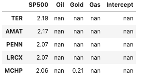
The security with the highest SP500 beta – TER

df_all_Betas[df_all_Betas['SP500'].notnull()].sort_values(by='SP500', ascending=False).head()

TER, with a Beta of 2.19, is the most volatile compared to the index and is a sign that if this index returns were to increase by some amount, e.g. 10% then the returns on this would be expected to increase by 21.9% (10% X 2.19), however if the index dropped by 10% then we would expect the return of TER to drop by -21.9%.

The security with the lowest GOLD beta – DLTR

df_all_Betas[df_all_Betas['Gold'].notnull()].sort_values(by='Gold', ascending=True).head()

DLR has a negative beta against gold, -0.43, a sign that its returns are negatively correlated to those of GOLD. If the return of DLR increased by the same 10% then we would expect the return on GOLD to drop by -4.3% (10% X -0.43), and vice versa. A decrease in the performance of DLR would often see a corresponding increase in the return of GOLD.

A beta higher than 1 is often seen as a risker investment, higher risk but also higher rewards, however it is a double-edged sword with a higher chance of underperforming a market.

• Vary the contents of the basket, for example include bonds, other indices, derivatives etc.
• Vary the model, for example, polynomial regression, nearest-neighbours regression
• Construct a cube of results with dimensions: security X model X basket

Finally, there are some more advanced pre-processing steps that can be carried out, for example testing for the existence of heteroscedasticity in the data.