Read time:
15 minutes
Data Intellect
Introduction
There are many tools available to load and manipulate data but this blog focuses on two – Alteryx (a user-friendly visual data analytics tool) and Pandas (a widely used Python package). Alteryx does not require a lot of programming knowledge to use, allowing beginners to get up to speed with it quickly. Alteryx consists of tools which users can drag and drop onto the canvas. Each tool has a specific function (for example the sort tool is used to sort data in ascending or descending order) and input and output anchors are used to connect to other tools in the workflow.
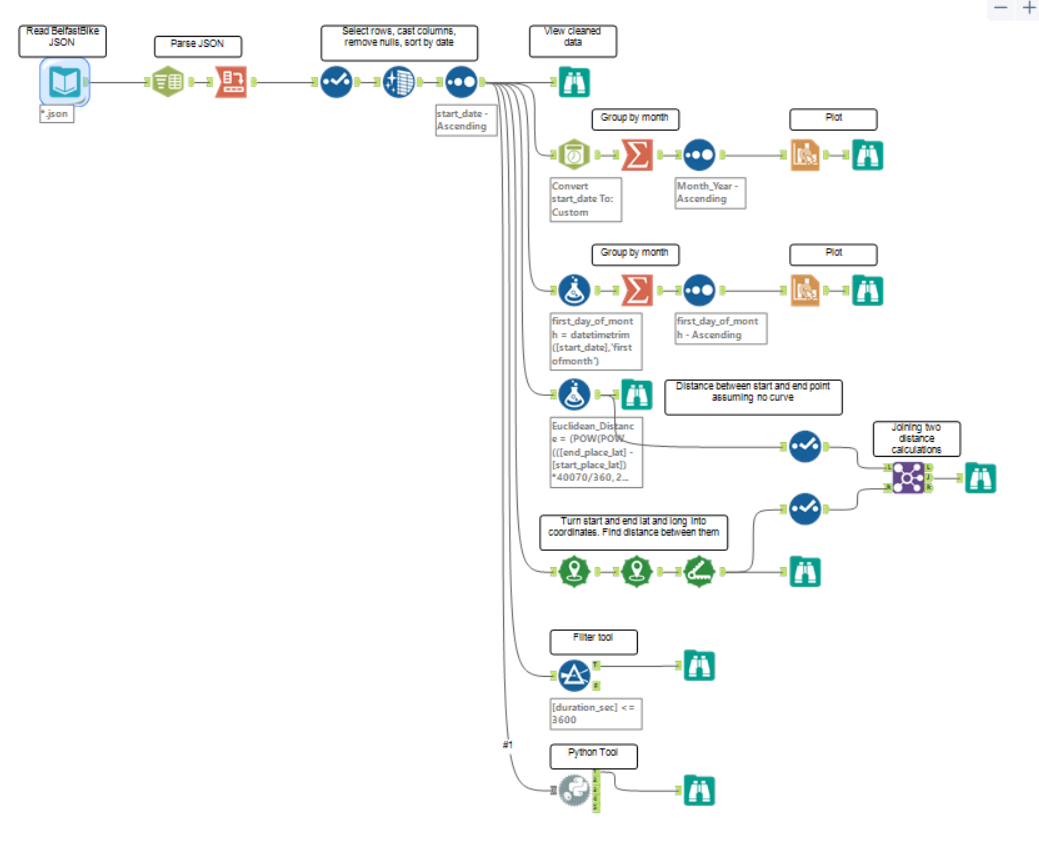
This blog will go through a simple Alteryx workflow and provide a comparison in Python using Pandas, Matplotlib and several other Python packages. The aim is to give a direct comparison between the two methods focusing on performance and ease of use. Below is a screenshot of the completed Alteryx workflow showing the initial data input and cleaning at the top left and each task on the right.
Data Input
The data used for this comparison is the Belfast Bike dataset which is freely available for anyone to download from Belfast Bike Historical Data in XML and JSON format. Each file contains one month of data and JSON files from March 2015 to November 2021 were used. The raw data was left untouched after it was downloaded and read directly into Alteryx and Python, resulting in the first problem – how to get over 80 JSON files into a single Alteryx table and Pandas DataFrame without reading them in one by one?
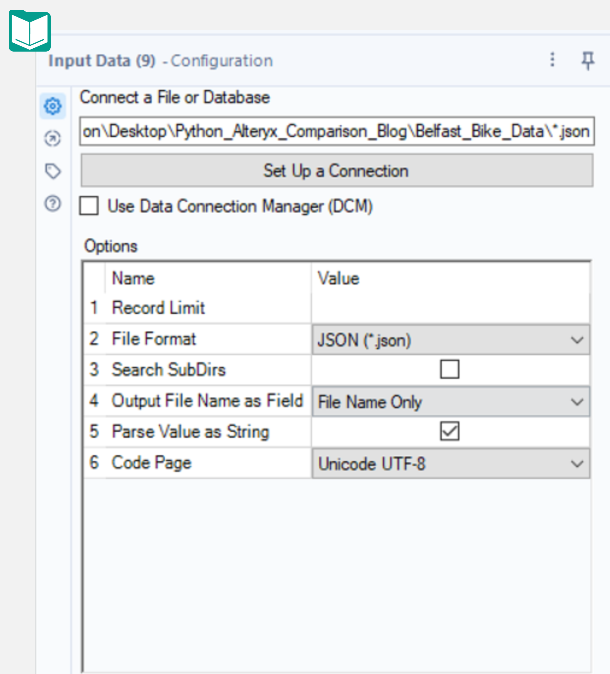
In Alteryx, you could use the Input tool and pass in the path to the folder containing the JSON files, appending \*.json to the file path. Surprisingly, this works (sort of). What Alteryx returns is a table with two columns:
1. JSON_name
2. JSON_ValueString
For a dataset which should have over 20 columns, this is obviously an issue. Alteryx has placed all of the field names in a single column and all of the values in another column. This requires a couple of extra tools to fix but first, the JSON_name column has an integer prepended to each column name, corresponding to the row number for each record in a JSON file. This number combined with the file name can be used to uniquely identify each record across all the JSON files.
The first step to correct this issue is to select “File Name Only” for the “Output File Name as Field” option in the Input tool configuration. Running the workflow again will add this extra column.
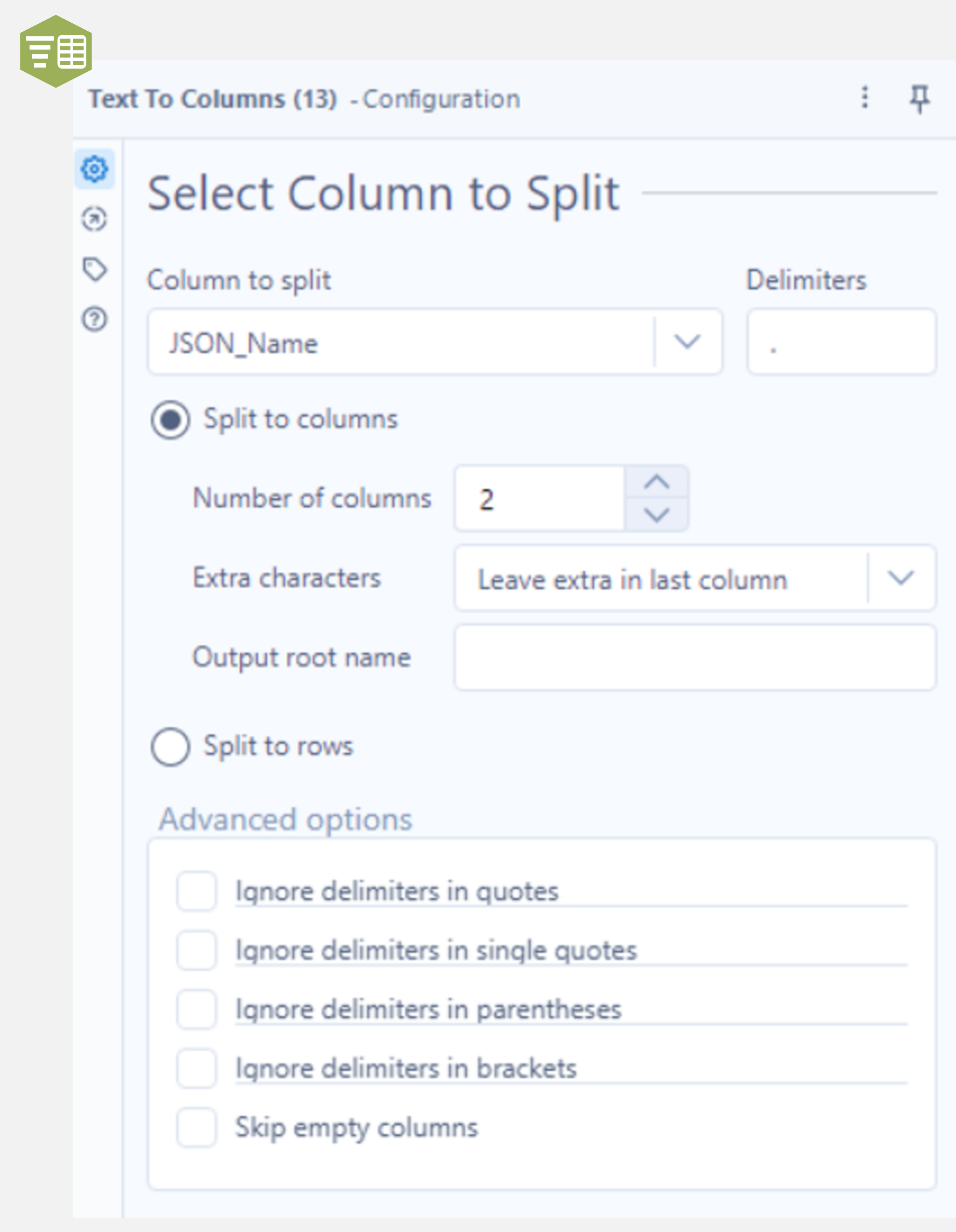
Next, add the Text to Columns tool to the output anchor of the Input Data tool, select JSON_Name as the “Column to split” and use a decimal point as the delimiter. Make sure “Split to columns” is checked, with the number of columns set to 2. Running this workflow and examining the output shows two extra columns (named 1 and 2) with the prepended integer in one and the remainder of the field name in the other.
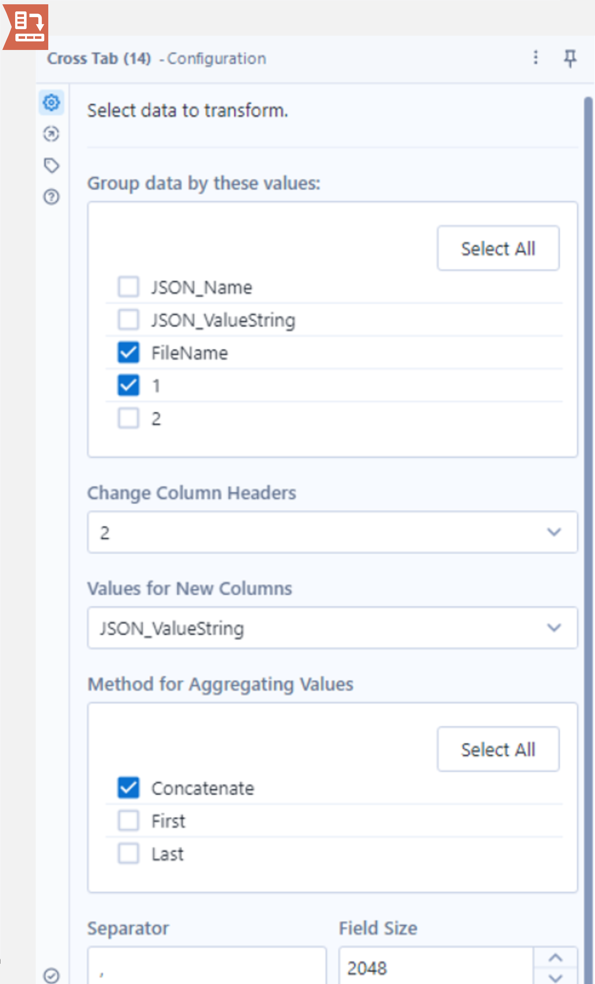
The final step involves using the Cross Tab tool. Attach this to the output anchor of the Text to Columns tool and take a look at the configuration panel. The first section allows users to select which fields to group on. Make sure to select both FileName and “1”. The “1” field contains the integer that was initially prepended to the field names in the JSON_Name column. Recall these two values uniquely define each row which is why both must be selected.
Next, set Change Column Headers to column “2” as this column contains the field names to set as the new column names. Finally, set “Values for New Columns” as JSON_ValueString and select one of the aggregation methods below (the rows have been uniquely defined so these aggregate methods are not expected to be used, however, it is still a required field).
Running the workflow gives a table in the correct format with a little over 1.2 million records. There are more steps than you might expect to get the Belfast Bike data into Alteryx given its batch loading capability but this is largely down to the file type used (JSON) and this process would be a lot simpler when reading in a CSV file.
Now for the same task in Python using Pandas. The first step is to get a list of all the JSON files in the directory where they are stored. Next, loop through the filenames, using the read_json method and concatenate the DataFrames using pandas.concat. Pandas’ read_json method can correctly interpret the JSON files automatically, returning the DataFrame with 1.2 million records.
import os
import json
import pandas as pd
from tqdm import tqdm

# path to json files
path = '..\\Belfast_Bike_Data\\'

# list of json files
json_files = [file for file in os.listdir(path) if file.endswith('.json')]

# reading json files to a single DataFrame
df = pd.concat([pd.read_json(path+file) for file in tqdm(json_files)], axis=0)
In Alteryx, the Input tool took 20.7 seconds initially but only 2.3 seconds when caching was used. The Text To Columns tool took 8.9 seconds and the Cross Tab tool took 71.5 seconds giving a total of 82.7 seconds when caching the data and 101.1 seconds when the data is not cached. When running the equivalent code in Python, the process took 28.7 seconds.
Cleaning Data
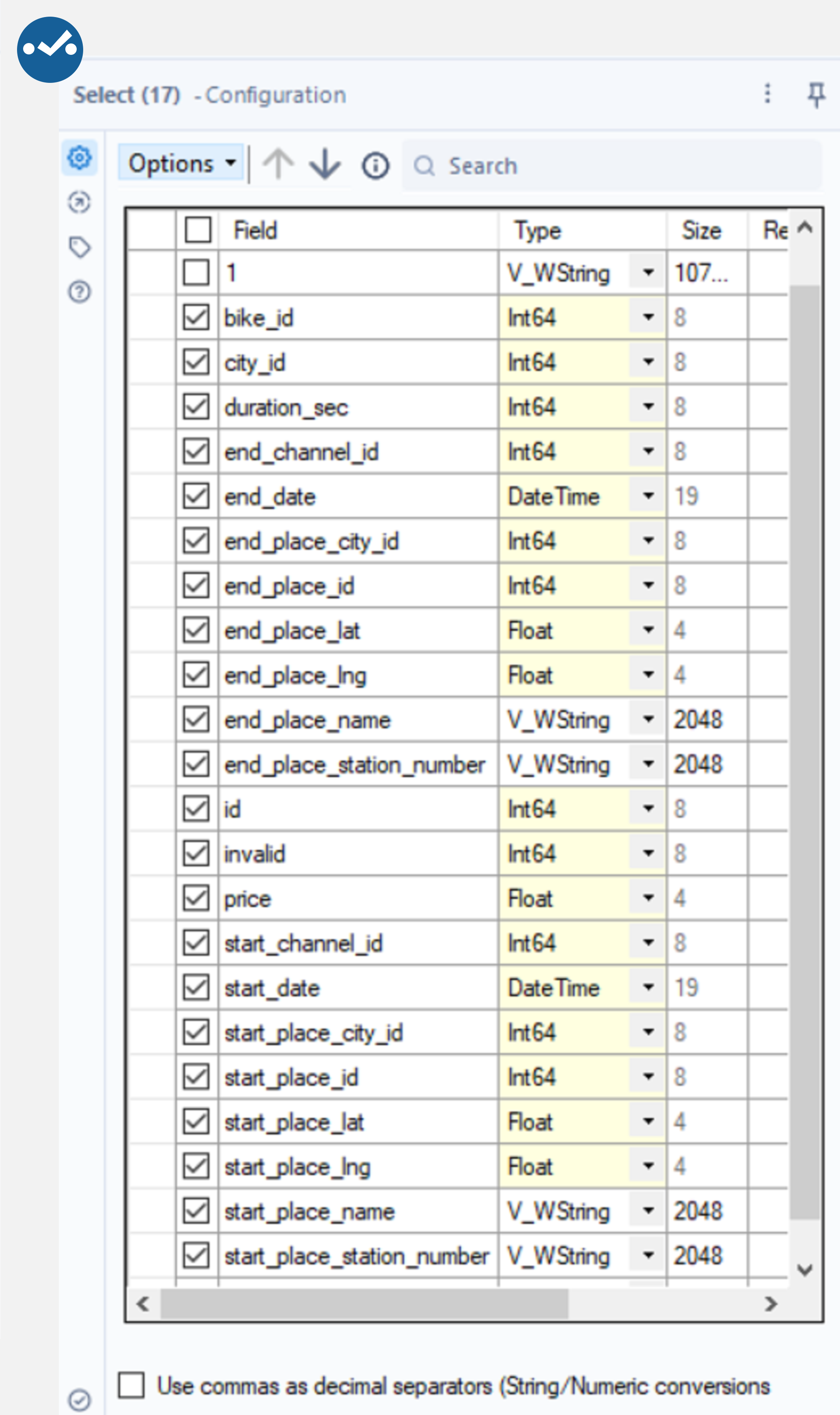
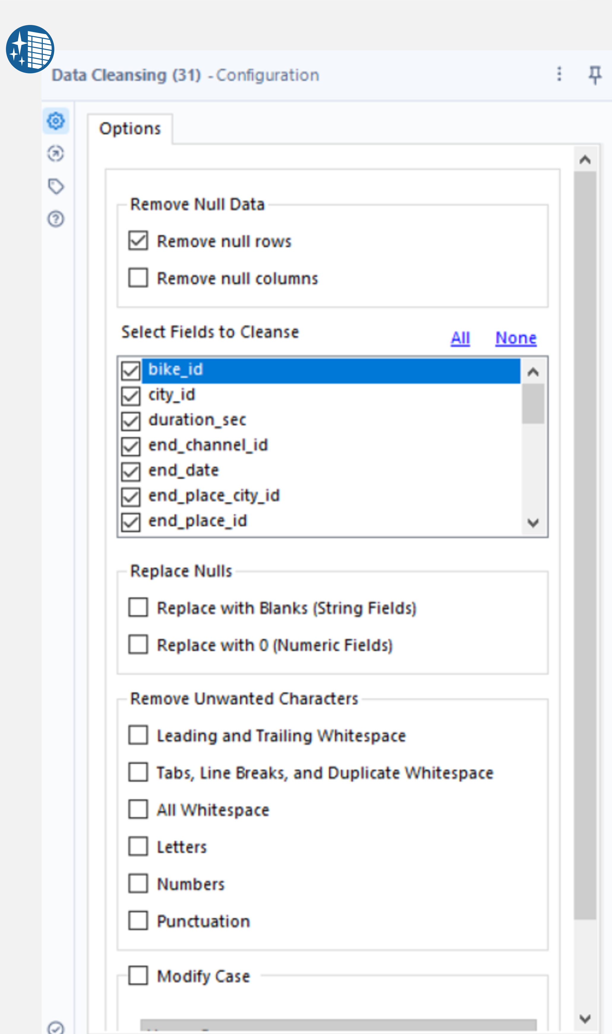
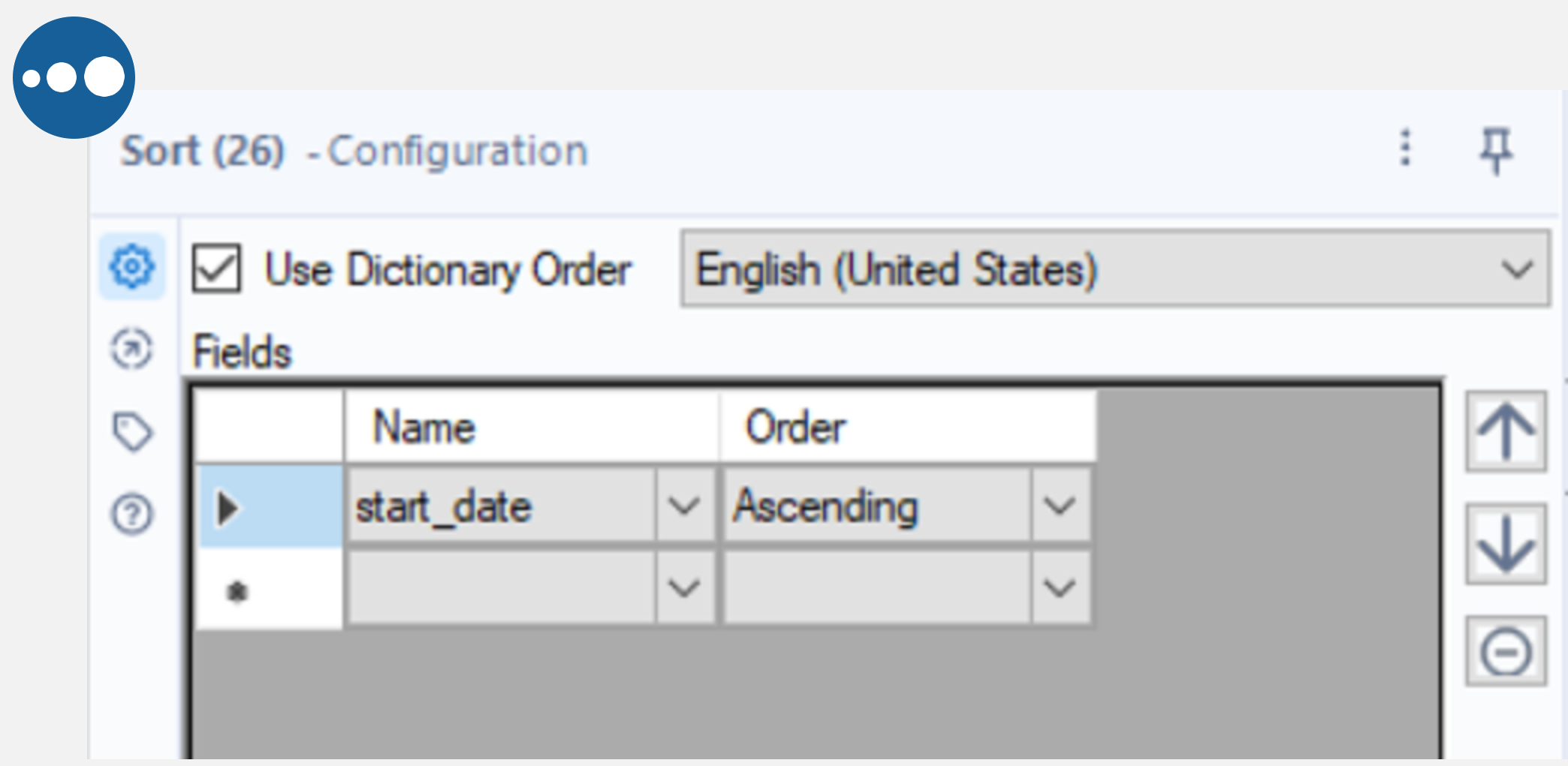
Alteryx has several tools to manipulate data. Here is an example of dropping columns and changing their data type using the Select tool, removing null rows using the Data Cleansing tool and sorting by a field with the Sort tool.
Connect the Select tool to the output anchor of the Cross Tab tool and deselect the “1” and FileName fields. Next, set the type to string or int64 where necessary and DateTime for the start and end dates. By connecting the Data Cleansing tool to the output anchor of the Select tool, the Remove null rows box can be selected to remove any null records from our data (where all fields are null). Finally, add the Sort tool to the output anchor of the Cleansing tool and sort by start_date ascending.
 |
 |
To achieve the same result in Python, the start and end date fields can be converted to datetime using pandas.to_datetime and sorted using the sort_values method shown below. Pandas will automatically select the appropriate data type for the remaining columns. To remove rows where all values are null, use the dropna method with how=’all’ to specify that only rows where all values are null are to be dropped.
# convert date columns to datetime
df['start_date'] = pd.to_datetime(df.start_date)
df['end_date'] = pd.to_datetime(df.end_date)

# sort by start date
df.sort_values(by='start_date', inplace=True, ignore_index=True)

# remove records where all fields are null
df.dropna(how='all',inplace=True)
In Alteryx, the Select tool took 3.6 seconds to run, the Data Cleansing tool took 36.9 seconds and the Sort tool took 2.8 seconds. In Python, the to_datetime method took 2.1 seconds to run, sorting the values took 0.4 seconds and removing nulls took 1.3 seconds.
Resampling and Summarize
This exercise involves down sampling the data to find the monthly total number of rentals. In Python, this can be done easily by using Pandas’ resample method as shown in the cell below.
# resample by month, finding the average number of rentals per month
df_monthly = df.resample('M', on='start_date').agg({"id":'size'}).rename(columns={'id': 'numrows'})
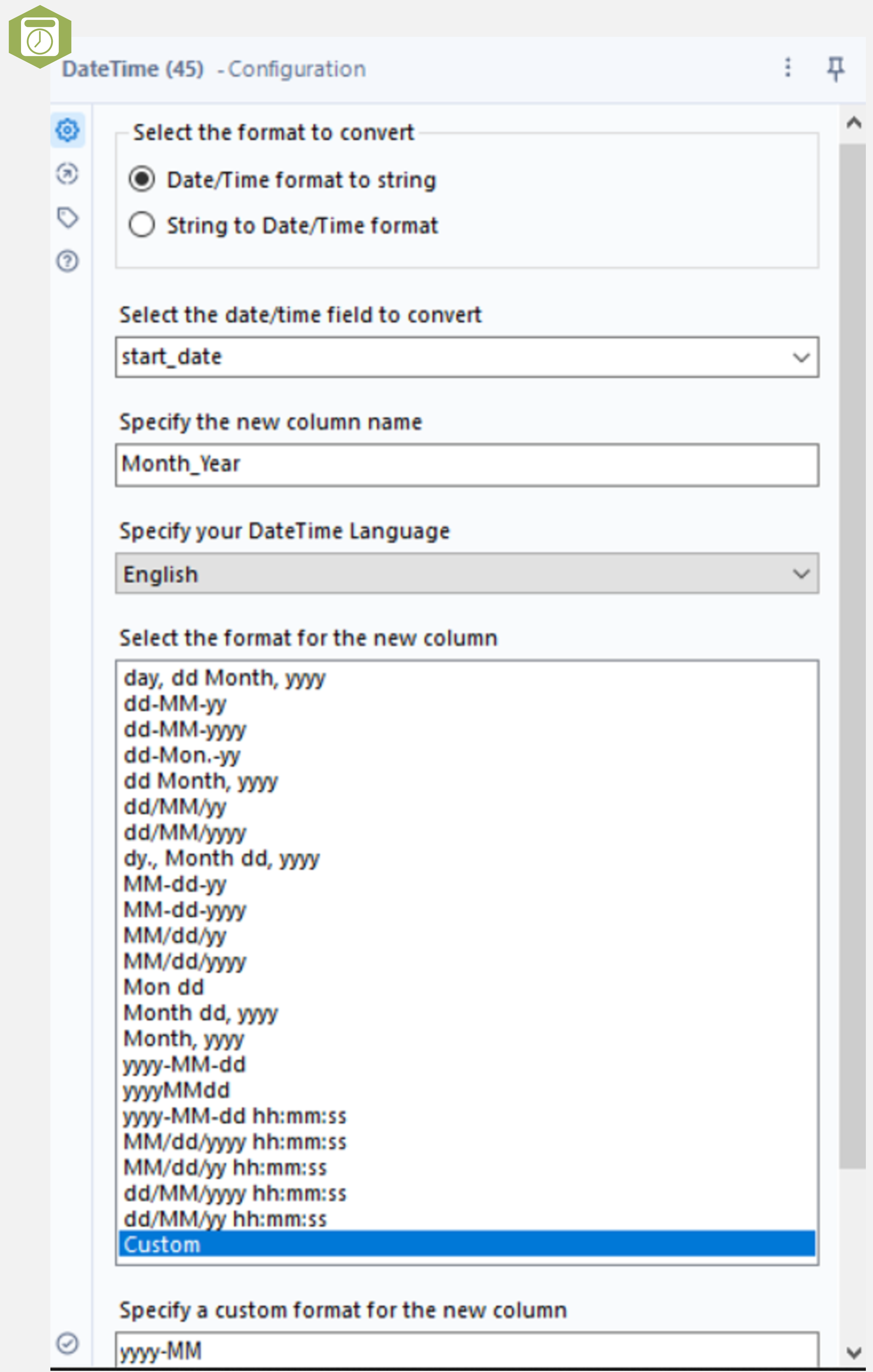
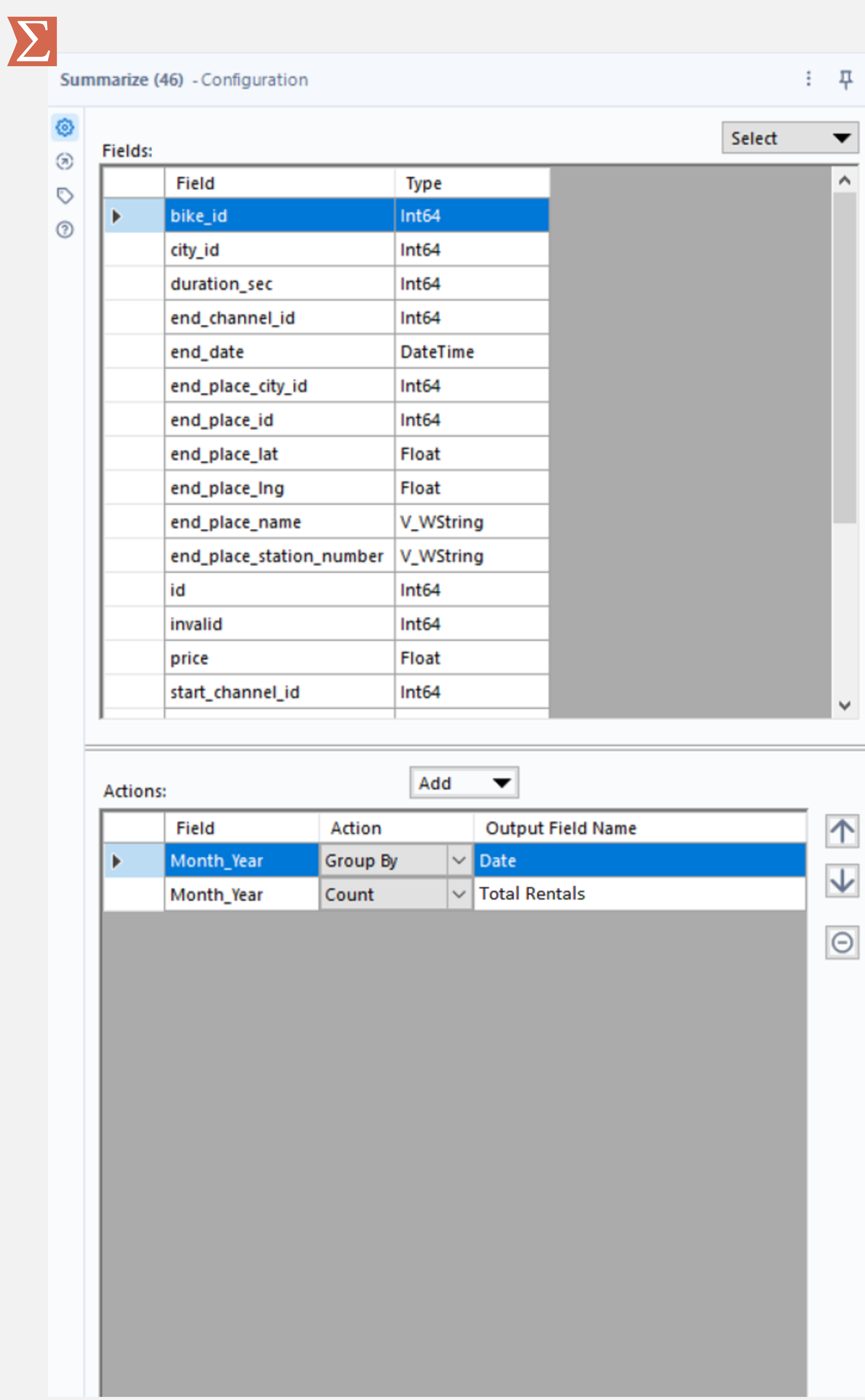
The same task in Alteryx requires a couple of extra steps. First, use the Datetime tool to select the month and year of the start_date only (using a custom format to put the year first, yyyy-MM). The Summarize tool can then be used to group on this new field and count the records. Finally, use the Sort tool to sort by the grouped column.
 |
 |
The Python option here is unsurprisingly quicker as it uses a single method, taking 0.1 seconds. The same process in Alteryx (date formatting and the Summarize tool) took 1.4 seconds for the formatting and 0.7 seconds for the Summarize tool.
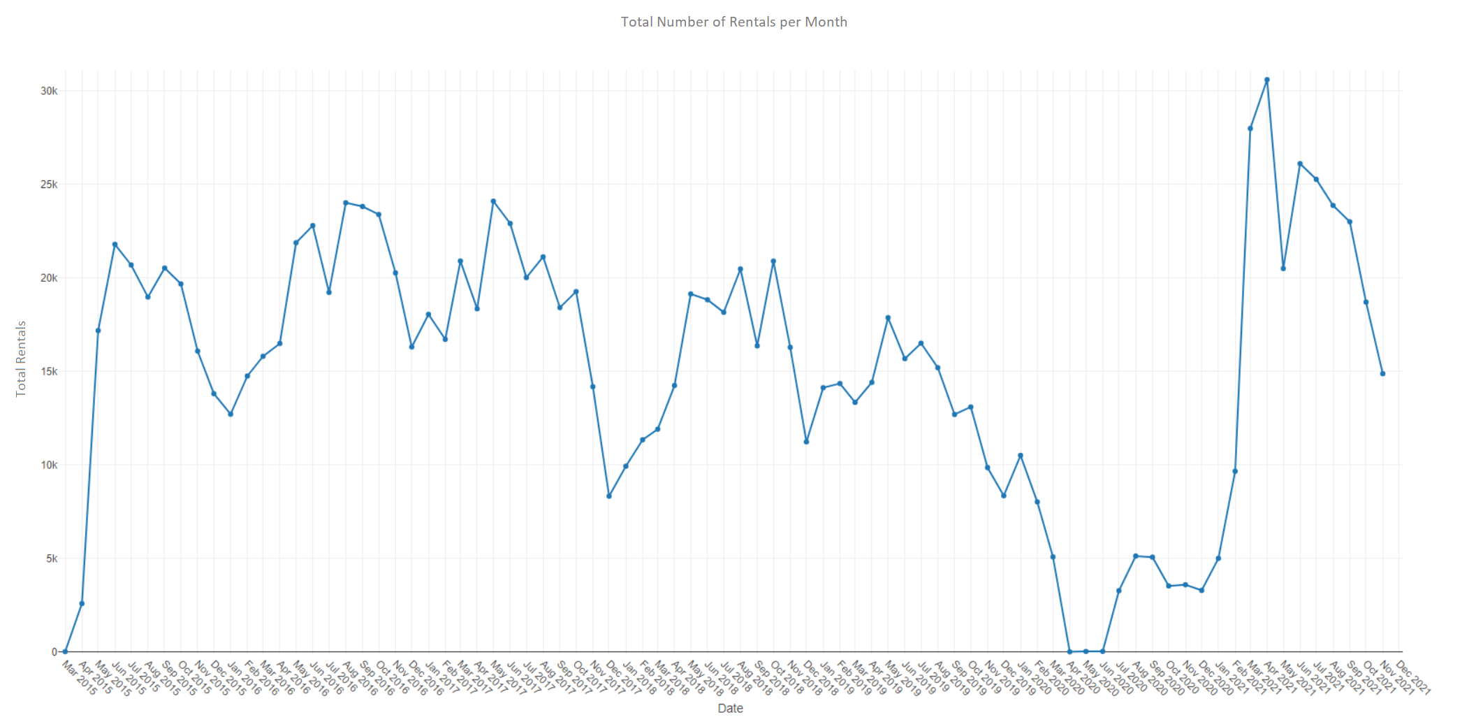
Plotting
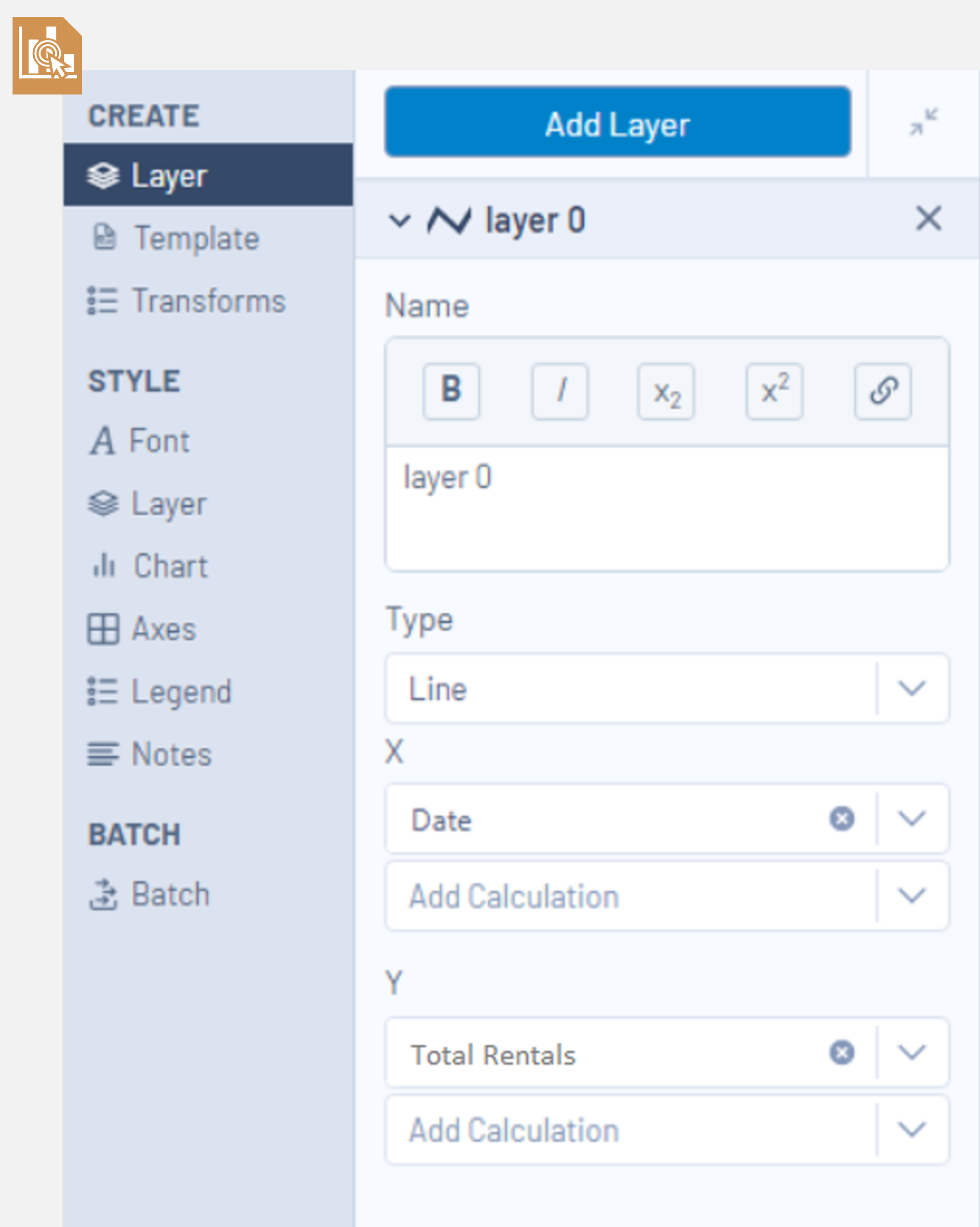
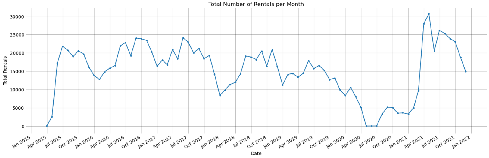
The next task is plotting the total number of transactions (number of bike rentals) for each month in the dataset. In Alteryx, this is done using the Interactive Chart tool. Select configure chart, create layer and select the reformatted Date column as the x values and the Total Rentals column as the y values. In the style section, lines and points can be shown by selecting both tick boxes in the layer tab. Further chart formatting can be done using the style settings including showing a grid, adding a title and altering x and y axis titles.
Plotting in Python can be done using Matplotlib. The cell below shows how to create a figure, plot the values and do some formatting. This is the first exercise where Alteryx is marginally quicker than Python (0.1 seconds vs 0.2 seconds).
import matplotlib.pyplot as plt
import matplotlib.dates as mdates

# plot total rentals against date
fig = plt.figure(figsize=(15,5))
ax1 = fig.add_subplot()

# x axis formatting
myFmt = mdates.DateFormatter('%b %Y')
ax1.xaxis.set_major_locator(mdates.MonthLocator(interval=3))
ax1.xaxis.set_major_formatter(myFmt)

fig.autofmt_xdate()
alpha = .3

ax1.plot(df_monthly.index, df_monthly.numrows.values, zorder=2, marker = '.', markersize = 5, linestyle = '-')

ax1.grid(zorder=1, color='black', alpha=alpha)
for spine in ['top', 'bottom', 'right', 'left']: ax1.spines[spine].set_visible(False)
ax1.tick_params(axis='x', which='major', color=[0, 0, 0, alpha])
ax1.tick_params(axis='y', which='major', length=0)

ax1.set_title('Average Number of Rentals per Month')
ax1.set_xlabel('Date')
ax1.set_ylabel('Mean Rentals')

fig.tight_layout()
A comparison between the Matplotlib and Alteryx plots is shown below. Both plots look very similar, however the nature of the formatting options with both tools introduces some subtle differences.
Additional Fields (Distance Calculations)
This section compares adding additional fields to the Alteryx table and Pandas DataFrame. For this example, the coordinates columns for the start and end locations were used to calculate a distance between them.
First, the Euclidean distance is calculated using Pythagoras’ Theorem. In Alteryx, connect a Formula tool to the Sort tool from the Cleaning Data section and add a new column “Euclidean_Distance“ in the configuration window. In the formula section, write an expression (shown below) which will be used to calculate this distance. This expression converts the difference between the latitude and longitude coordinates into a distance using Earth’s circumference and Pythagoras. Anchoring a Browse tool to the Formula tool allows users to see the results.
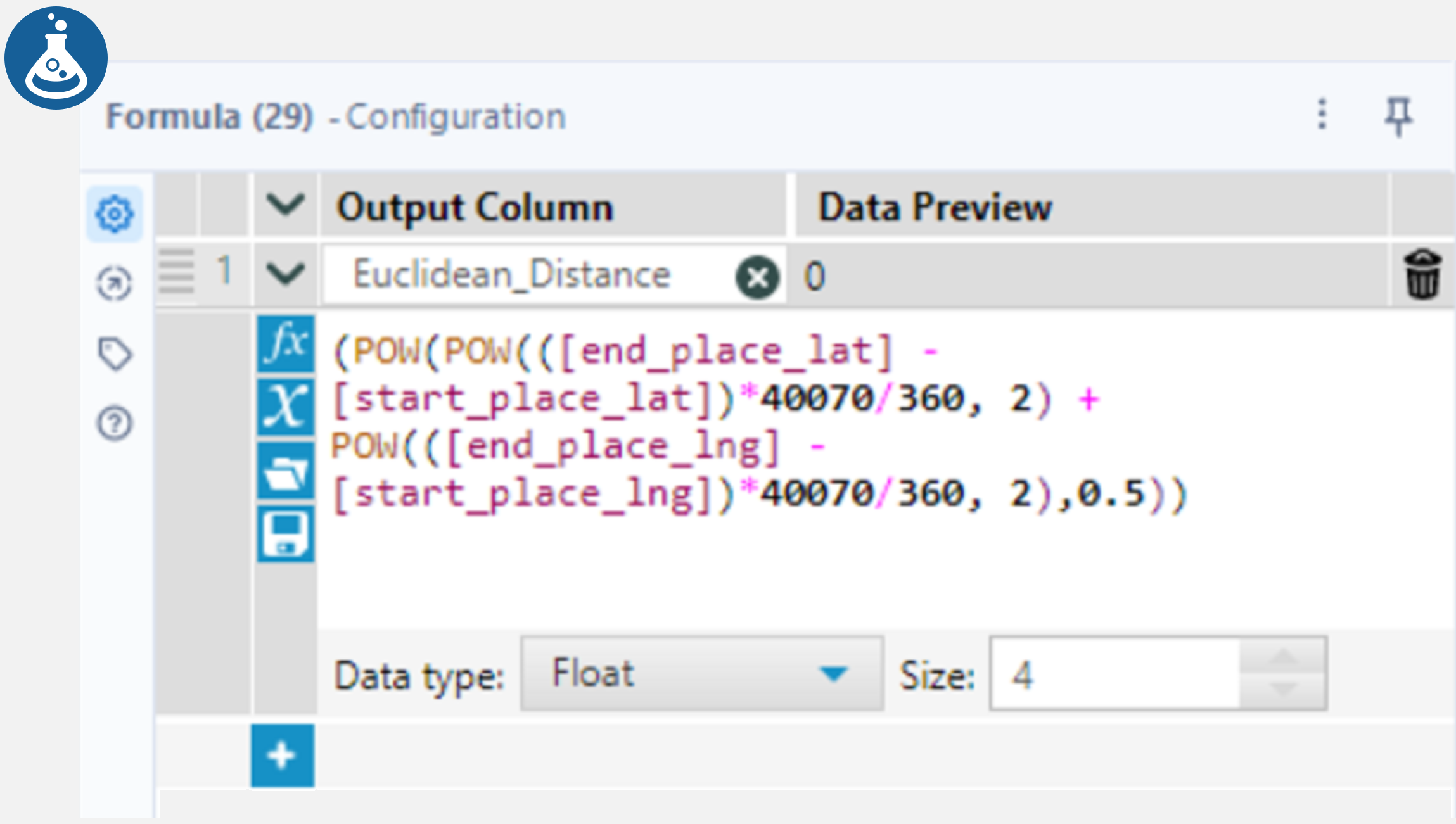
The method for calculating this distance in Python is very similar to the above Alteryx method. Python can also use the pow() method (although the Python code below uses ** instead). The rest of the expression is very similar between Python and Alteryx, however, the field names are referenced differently when using Pandas. This expression is assigned to a new column in the DataFrame as shown in the cell below.
# earth's circumference divided by 360 degrees (rough distance of 1 degree of latitude or longitude)
km = 40070/360

# use Pythagoras to calculate distancebetween start and end point
df['Euclidean_Distance'] = (((df['end_place_lat'] - df['start_place_lat'])*km)**2 + ((df['end_place_lng'] - df['start_place_lng'])*km)**2)**.5
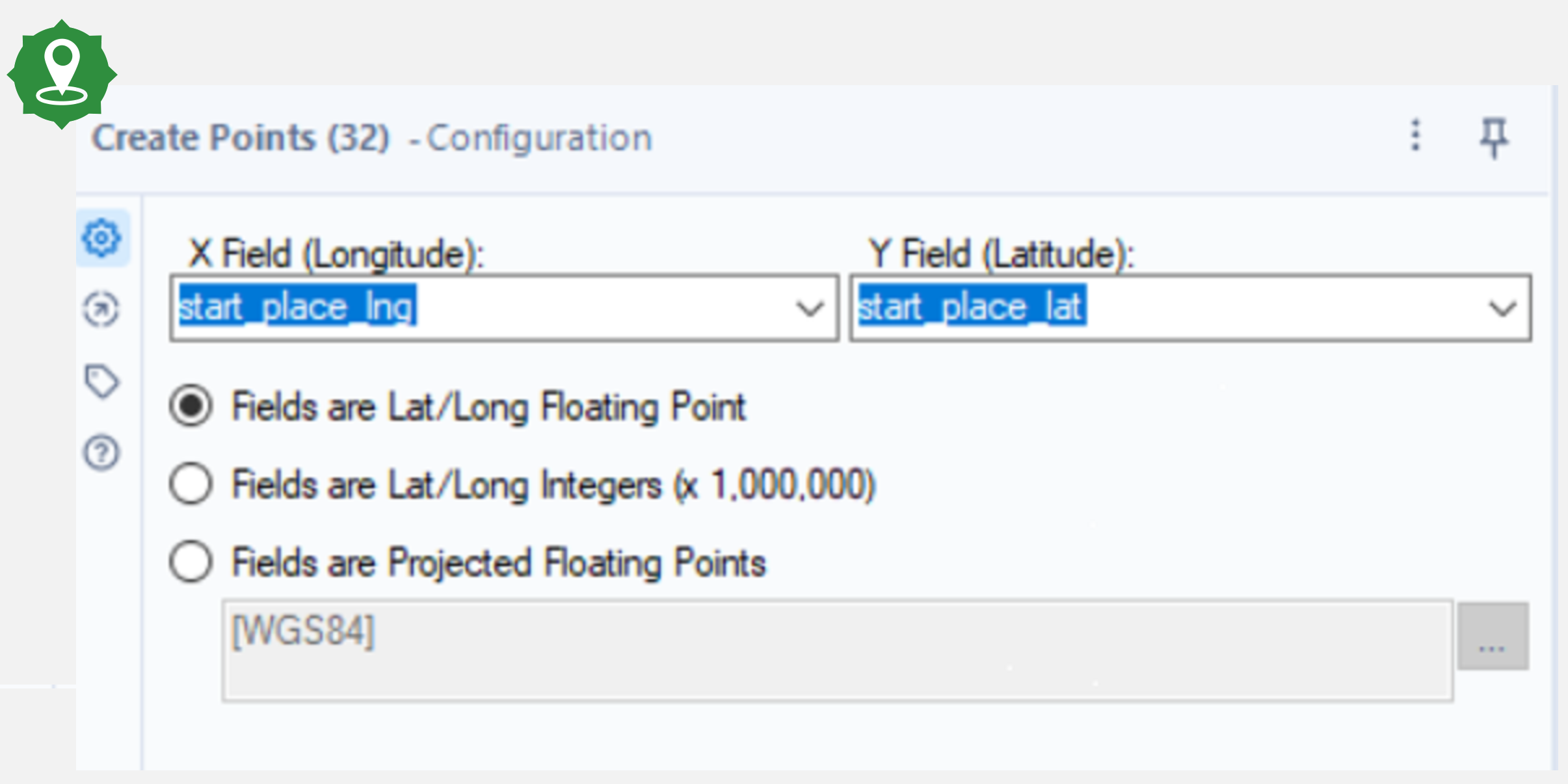
To make these calculations more accurate, the distance between the coordinates taking into account Earth’s curvature was found. In Alteryx, this is done using the Create Points and Distance tools. Connect the Create Points tool to the output anchor of Sort tool from the Cleaning Data section and select the start place latitude and longitude in the drop down menu. The fields here are floating point latitudes and longitudes. Connect another Create Points tool to the output anchor of the first Create Points tool and repeat the process for the end point coordinates.
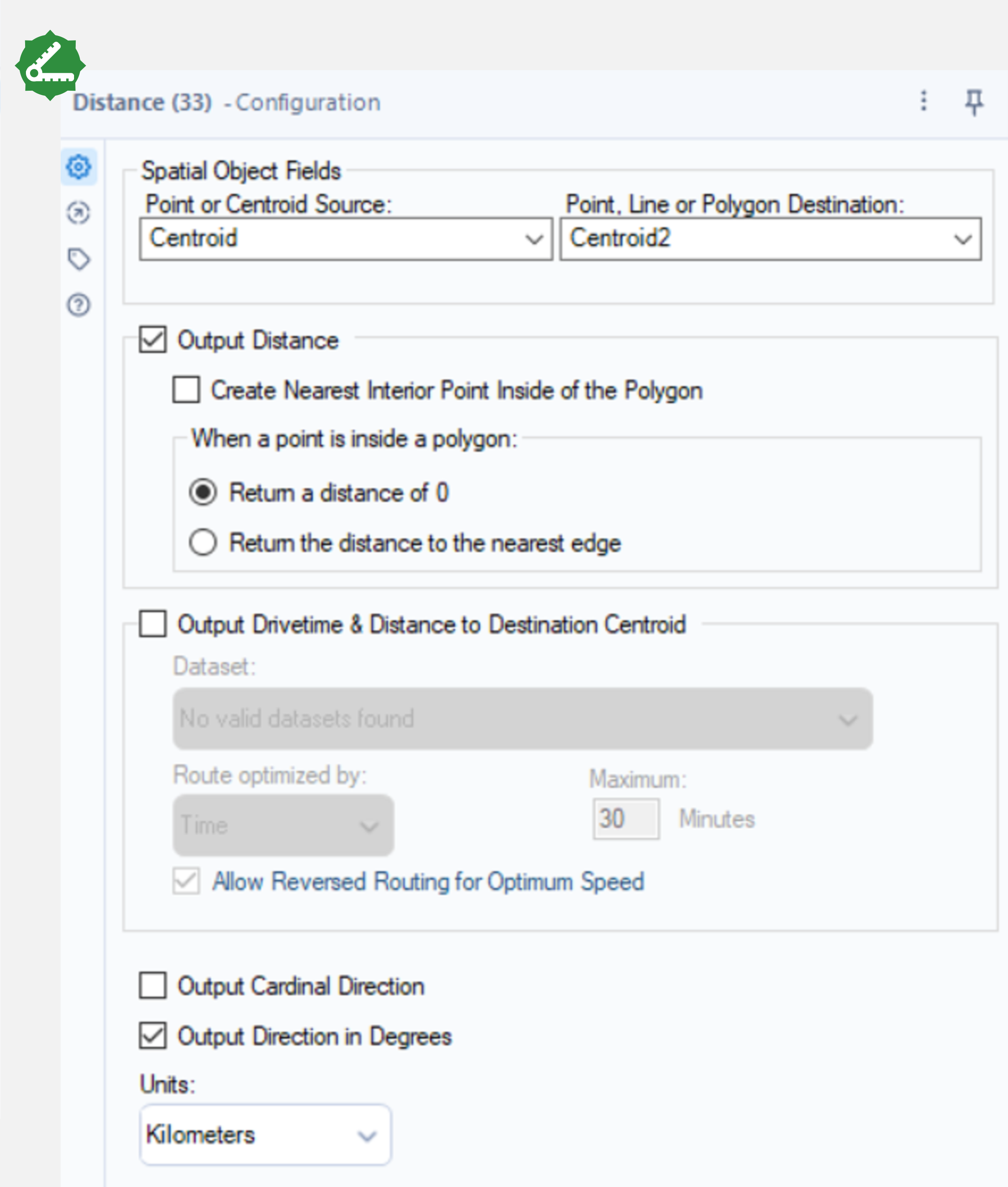
For the next step, use the Distance tool to calculate the ellipsoidal distance between the two points (an accurate distance model which assumes the Earth is an ellipsoid). Connect this tool to the output anchor of the final Create Points tool and select Centroid and Centroid2 as the points from the drop down menu in the configuration window and select Output Distance.
A similar process in Python can be done using Vincenty (install with pip install vincenty) to calculate the Vincenty distance as shown in the cell below. There are many other distance calculation tools available in Python from libraries such as Scipy or Geopy, however, Vincenty uses a similar distance algorithm to Alteryx’s distance tool.
from vincenty import vincenty

# create tuples for start and end coordinates
df['start'] = [(x,y) for x,y in zip(df.start_place_lat, df.start_place_lng)]
df['end'] = [(x,y) for x,y in zip(df.end_place_lat, df.end_place_lng)]

# calculate vincenty distance
df['Vincenty_Distance'] = [vincenty(start_loc,end_loc) for start_loc,end_loc in tqdm(zip(df.start,df.end))]
To calculate the Euclidean distance using the Formula tool, Alteryx took 1.2 seconds compared to Python’s 0.1 seconds using the same equation. Conversely, when calculating a more accurate distance, Alteryx was faster, taking 4.8 seconds to create the points and calculate the distance where Python took 25.6 seconds. There may be a Python package which can calculate this distance quicker than Vincenty, however, out of the several tools tested, this was the quickest.
Joining
This section covers a comparison in joining the two distance calculation columns from the section above. In Alteryx, first tidy each table by using a Select tool and only selecting the “id“ and respective distance column. Connect a Join tool to the output anchors of both of the Select tools and join on the “id“ column, making sure to select only one id column (but both distance columns) so there are no duplicates. Connecting a Browse tool to the “J” output anchor calculates an inner join for the tables. The “L” and “R” output anchors are used for left and right joins.
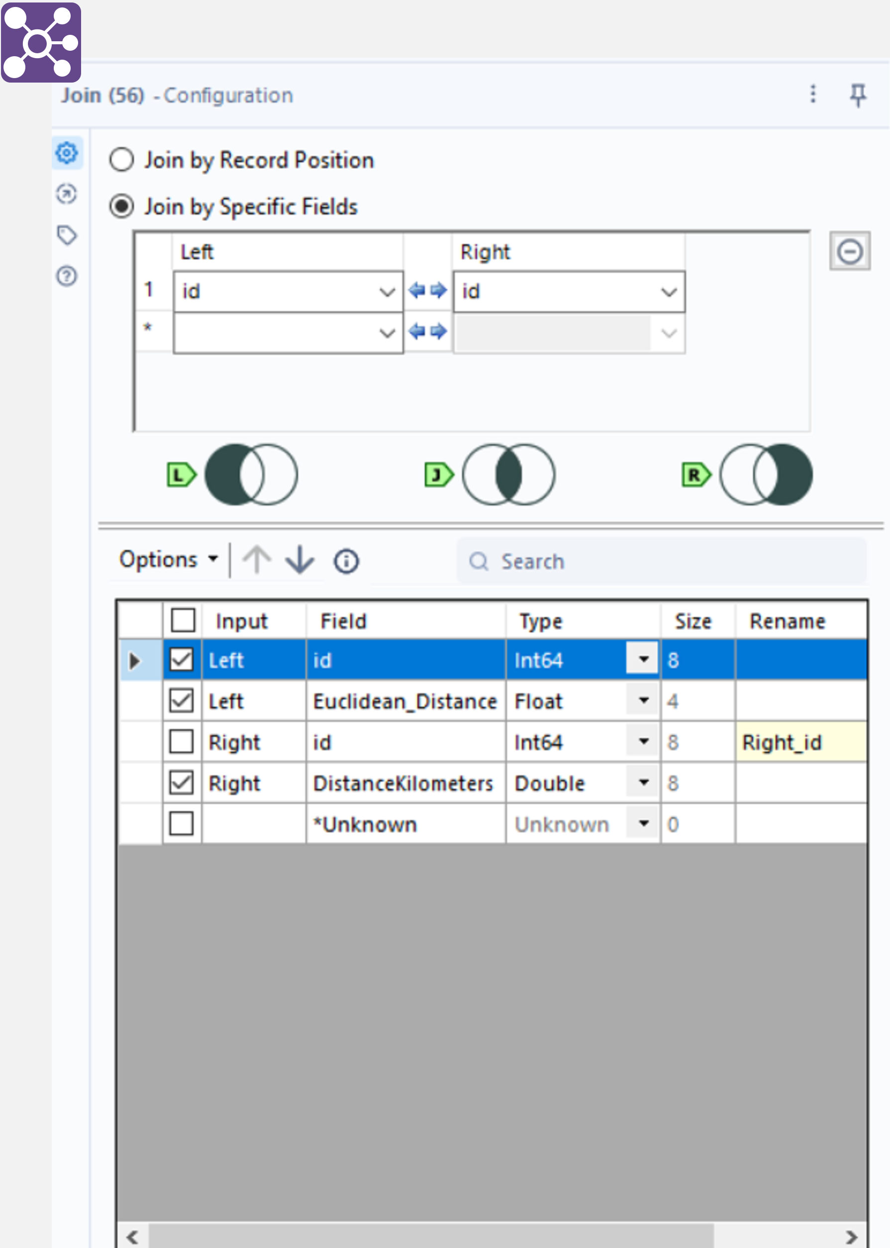
In Python, a similar result can be achieved by using the merge method as shown below. Here, the different distance columns are split into two separate DataFrames with the id as the common field to join on. Python was quicker with 0.9 seconds for a merge compared to 3.3 seconds for an Alteryx join.
# pandas merge
df[['id', 'Euclidean_Distance']].merge(df[['id', 'Vincenty_Distance']], how='inner',on='id')
Filtering
Filtering is the removal of records based on one or more conditions. In Alteryx, this can be done with the Filter tool. Connect this tool to the Sort tool used in the Data Cleaning section and select “Basic filter” in the configuration window. Next, select the column to filter on (duration_sec) and <= 3600 for the condition. This tool provides two separate output anchors, one for when the condition is met and one for when it is not. Connect a Browse tool to the “T” (true) output anchor and note how there are less rows than before as all records greater than 1 hour in duration have been removed.
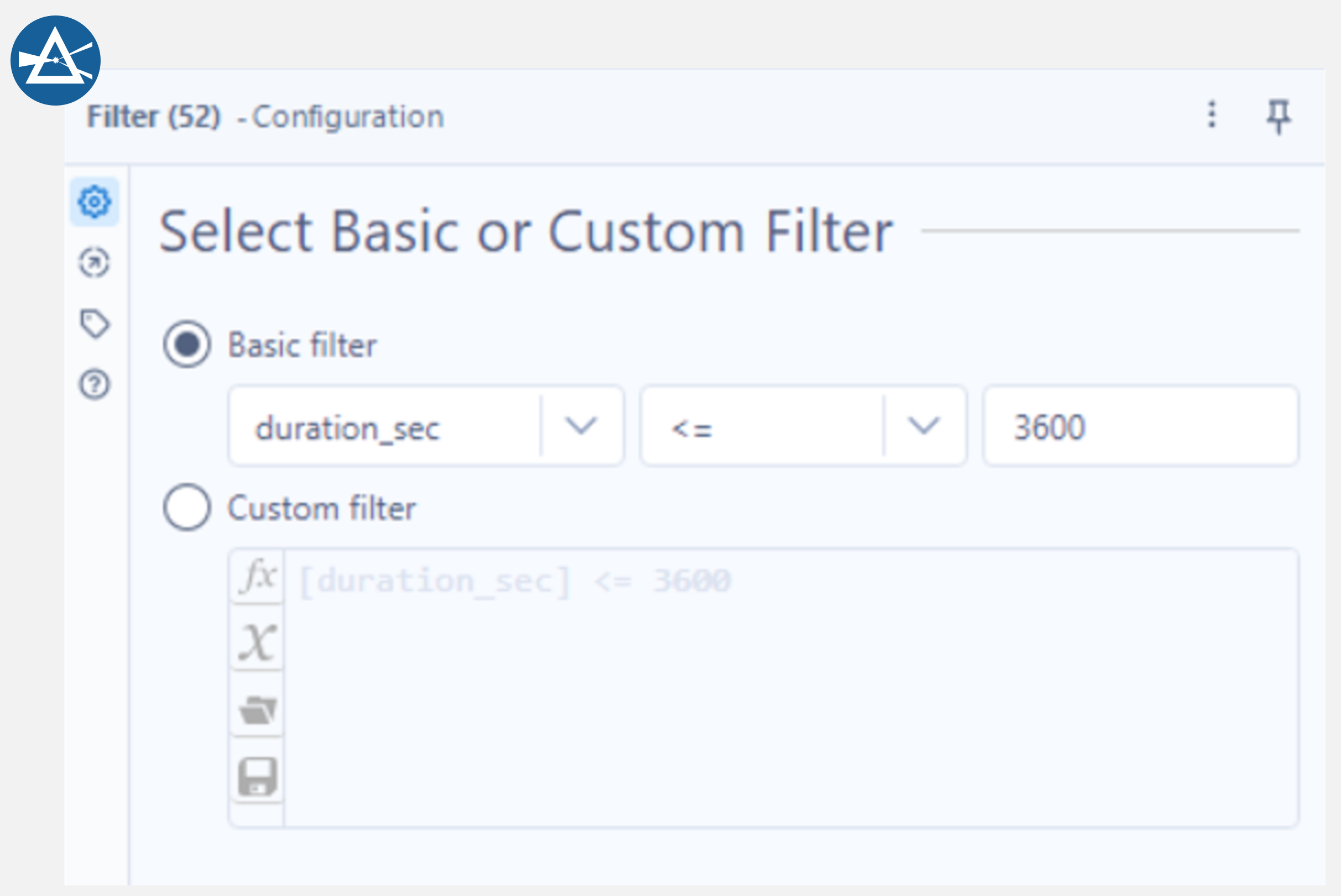
Filtering a DataFrame in Python using the same condition as described in Alteryx above is equally as easy and is shown in the cell below. Both processes took the same time in Python and Alteryx – 0.1 seconds.
# filter for records with a duration less than 1 hour
df[df.duration_sec <= 3600]
Alteryx Python Tool
Alteryx has a tool for plotting histograms, however, the version of Alteryx that was used for this test did not have it installed. This was disappointing but also a good opportunity to use the built in Python tool in Alteryx to plot the histogram instead. Connect this tool to the output anchor of the Sort tool used in the Data Cleaning section and a Jupyter notebook will appear in place of a configuration window. The first step is to import the necessary libraries shown below.
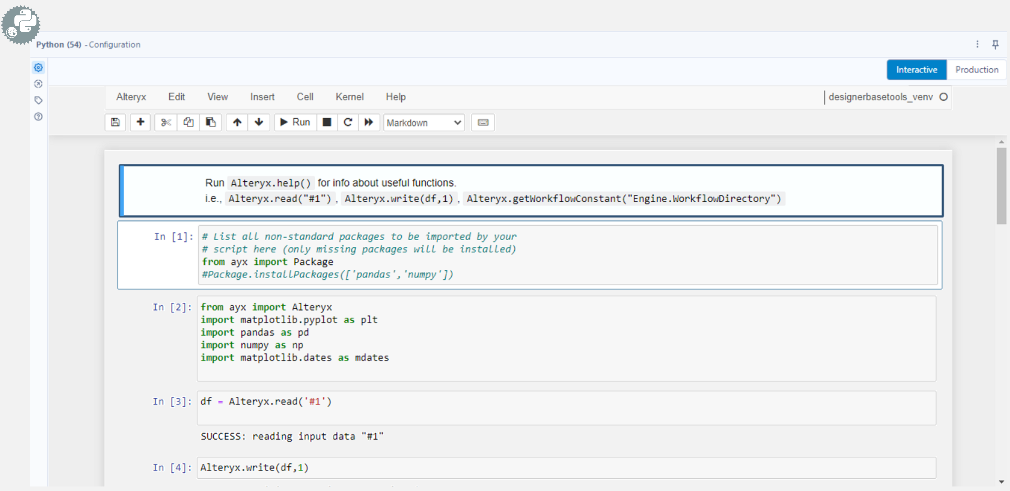
To get the data into a Pandas DataFrame in this notebook, use Alteryx.read (as shown in the cell above). This method takes “#1” as an argument (the input anchor shows the incoming data as #1). To output the data back to Alteryx, write it to one of five output anchors using the Alteryx.write method. Connecting a Browse tool to output anchor 1 returns the data passed to Alteryx.write. The histogram can be plotted using the code in the cell below.
import numpy as np
# plot histogram of rental frequency throughout the day
fig = plt.figure(figsize=(15,5))
alpha = .3
time = pd.to_datetime(df['start_date'].dt.time, format='%H:%M:%S')
ax2 = fig.add_subplot()
ax2 = time.hist(bins=24, figsize=(10,5), grid=False, edgecolor='white', zorder=2, weights=np.ones(time.size)/time.size)
ax2.xaxis.set_major_formatter(mdates.DateFormatter('%H:%M'))
ax2.yaxis.set_major_formatter('{x:.1%}')
ax2.grid(axis='y', zorder=1, color='black', alpha=alpha)
ax2.spines['bottom'].set_alpha(alpha)
for spine in ['top', 'right', 'left']: ax2.spines[spine].set_visible(False)
ax2.tick_params(axis='x', which='major', color=[0, 0, 0, alpha])
ax2.tick_params(axis='y', which='major', length=0)
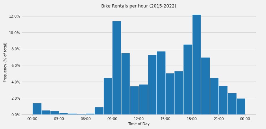
ax2.set_title('Bike Rentals per hour (2015-2022)')
ax2.set_xlabel('Time of Day')
ax2.set_ylabel('Frequency (% of total)')
fig.tight_layout()
The plot below shows the histogram produced in the Python tool and is identical to the same code run in a local Jupyter notebook.
The Python tool comes with several build in packages, found here, which can be imported as normal, however, it is also possible to install additional Python libraries using the Alteryx.installPackages method. This process took 16.4 seconds in Alteryx but pasting the cells into a Python notebook outside of Alteryx only took 4.9 seconds.
Conclusion
Hopefully this short introduction to Alteryx was helpful in determining its usefulness when up against Python. Alteryx’s drag and drop interface is very easy to get the hang of and is appealing to non programmers. Furthermore, the documentation available for Alteryx helps users get up to speed with these tools quickly, however, the trade off is Alteryx is generally slower to execute compared to the same task(s) in Python (with some exceptions such as the distance calculations). For example, running the full Alteryx workflow (with caching) took around 2 mins 30 seconds, however, the same workflow as a Python notebook ran in about 1 minute. Moreover, using the Python tool in Alteryx can fill in the gaps for any tools not found in Alteryx.
To summarise the results, the Alteryx Data Input tool allows for batch loading of files with the trade-off of needing extra tools to parse the JSON where Pandas can parse the JSON automatically. Additionally, Alteryx does not have a resample tool like Pandas, instead users must alter the date format to show only the month and year (if grouping by month) and use the Summarize tool to group by this reformatted date. Alteryx’s Join tool has output anchors for left, right and inner joins, allowing all joins to be completed simultaneously. Similarly, the Filter tool has output anchors for both the true and false outputs.
Finally, whilst Alteryx is easy to use for a complete beginner, Python is free and for anyone doing this kind of work often – worth learning how to use. Hopefully this workflow was easy enough to follow along both in Python and Alteryx and convinces some Python users to give Alteryx a go and vice versa.
| Alteryx Timings / s | Python Timings / s | |
|---|---|---|
| Data Input | 82.7 | 28.7 |
| Sort | 2.8 | 0.4 |
| Select and Data Types | 3.6 | 2.1 |
| Data Cleansing / Drop Nulls | 36.9 | 1.3 |
| Resample / Summarize | 2.1 | 0.1 |
| Plotting | 0.1 | 0.2 |
| Euclidean Distance | 1.2 | 0.1 |
| Ellipsoidal Distance | 4.8 | 25.6 |
| Join | 3.3 | 0.9 |
| Filter | 0.1 | 0.1 |
| Histogram | 16.4 | 4.9 |
Share this: