Dexter Lee
KDB-X introduces virtual tables as a way to build queryable tables over data that already exists on disk. Rather than loading a conventional partitioned database, a virtual table can be built over a set of existing data and presented to the user as a table.
That gives us another way to think about intraday data. In particular, we can rethink how the current day is stored and queried without having to keep the whole thing in an RDB.
This post explores that idea by building a small TorQ capture stack around virtual tables. The data is written to disk partitioned by instrument, with the directory structure carrying information that would normally live in a column. The reader can then query both historical and current-day data through a single virtual table.
Standard TorQ Architecture
A typical TorQ deployment for capturing and serving tick data has a few processes involved.
- A tickerplant to publish updates out
- A real time database that holds current day data in memory
- A write database that spools the same data to disk
- An intraday database that serves the data persisted by the write database
- At end of day, a sort process that merges that into the historical database, which then reloads.
The design works well, but there are three costs worth considering.
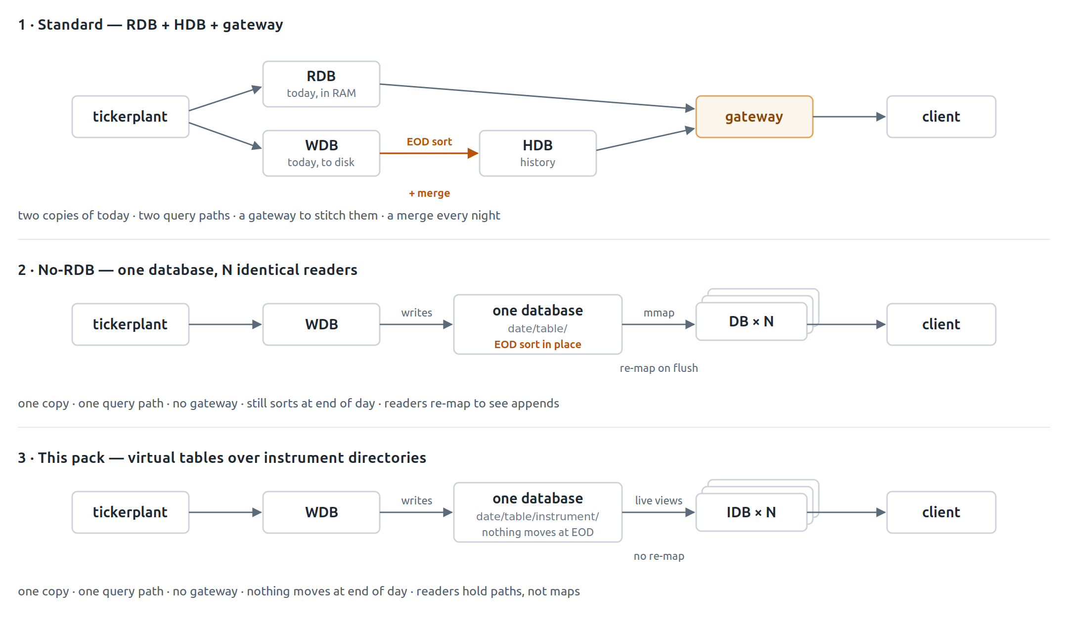
The live day can’t be indexed on disk. A p# attribute cannot be maintained on a table that is still being appended to, so every selective lookup against the live day on disk, such as through an IDB, has to scan the whole column. The usual solution is an RDB in memory for today and an HDB for history. That gives you two query paths, and a gateway to stitch the results together.
The day has to fit in RAM. The RDB keeps the whole day in memory, so the hardware has to be sized for the busiest day you expect rather than an average one.
End of day is expensive. The WDB output has to be sorted, given its attributes, merged into the HDB and then reloaded. That means a burst of I/O proportional to the day’s volume. The biggest days take the longest, and if something fails halfway through, you can end up with a partition that is only partly merged.
Removing the RDB
Matt’s no-RDB work takes a different approach: remove the RDB altogether. Its readers are TorQ’s own IDB processes, pointed at the whole database rather than just the WDB’s partition. If the writer writes into the database that the readers are already serving, there is nothing to stitch together. Multiple identical readers can memory-map the same tree and serve queries in parallel.
With the RDB gone, there is now one copy of the data and one query path. There is also no gateway sitting in front of the data and no need to budget a day-sized block of RAM.
There are still a few practical considerations around this approach, particularly around indexing the live day and keeping readers up to date with changes to the on-disk data.
- The live day is still un-indexed by default. No-RDB provides an opt-in index to address this, but each reader still needs to maintain its own copy of the indexed column in memory by relying on .Q.pm internals.
- End of day still sorts. Nothing moves between processes anymore, but the partition is still rewritten into a hidden copy, sorted, and then swapped back in. For a short time, that means the day takes up almost twice as much disk space.
- Readers need a way to pick up changes to live data. Matt’s approach uses .Q.MAP[] together with periodic reloads to refresh the latest data. This works well, but it also means the historical data needs to remain uncompressed, while the fast lookup path depends on undocumented .Q.pm internals that could change in the future.
This is where the virtual-table approach comes in.
Instead of storing the instrument as a column, it is saved as a directory. A filter on the instrument can then select which directories to open rather than scanning a column. The live day therefore doesn’t need an attribute, and there is no overnight rebuild just to add one.
Virtual tables also change what the reader needs to keep open. A partition opened with a trailing slash is a path, not a memory map, so q maps it afresh on each query. That is what makes an append visible because there is no mapping to go stale. This is already how kdb+ works by default. \l reads the layout but maps nothing, and without .Q.MAP[], each query maps what it needs. The reader therefore needs no reload, no .Q.MAP[], and no .Q internal to keep up with new data.
The brief
The idea is to build a small TorQ capture stack around virtual tables.
The pack should include: discovery, a segmented tickerplant, a write database splayed by instrument and flushing every second, a dummy feed to push data through the system, and an intraday database that can query both historical and current day data.
- End of day – Kept simple, the tickerplant rolls logs and the writer rolls to a new date directory.
- The reader – One process serves both historical and current day queries.
- Minimal processes – No gateway, no sort process, no sort workers and no RDB.
The instrument becomes a directory
With the instrument in the path, where sym=`AMD selects a directory instead of scanning a column.
var/db/
  2026.08.24/
    trade/
      AAPL/   time price size stop cond ex side
      AMD/    time price size stop cond ex side
    quote/
      AAPL/   time bid ask bsize asize mode ex src
Notice that sym isn’t one of the columns. It is represented by the directory name, so the query can tell what a directory contains without reading the data inside it.
If sym were still a column, finding AMD would mean opening the sym file in every directory, reading it and discarding the rest which is exactly what this layout is trying to avoid.
However, kdb+ cannot load this tree. Its partitioned-database machinery expects date/table/column so this is not a database it recognises.
Making this queryable is where KDB-X virtual tables come in. The rest of this post looks at how they work in practice.
A virtual table is a catalogue and a list of views
Unlike an HDB you load with \l, a virtual table is built. You tell KDB-X which partitions exist, hand it an open view of each one, and it gives you something that users can query like a table.
The function that builds it is mkP, from the kx.pq.t module that ships with KDB-X:
mkP:(use`kx.pq.t)`mkP
use resolves the module against QPATH and returns a dictionary of its exports. It is also what makes this design KDB-X-specific since use is a KDB-X function and will not run on kdb+ 4.x.
mkP takes a single dictionary. In the examples below, the key is called the catalogue and the value is called views.
The catalogue is a table with one row per partition, with the partition keys as its columns. Views is a list of opened partitions.
paths                                 / one per partition, trailing slash
`:/db/2026.01.01/trade/AAPL/
`:/db/2026.01.01/trade/AMD/
`:/db/2026.01.02/trade/AAPL/
catalogue:([] date:2026.01.01 2026.01.01 2026.01.02; sym:`AAPL`AMD`AAPL)
Views    :get each paths              / views is a reserved keyword
catalogue                             / a table, one row per partition
date       sym
---------------
2026.01.01 AAPL
2026.01.01 AMD
2026.01.02 AAPL

Views                                 / a list, one view per row
+`time`price`size`broker!`:/db/2026.01.01/trade/AAPL/
+`time`price`size`broker!`:/db/2026.01.01/trade/AMD/
+`time`price`size`broker!`:/db/2026.01.02/trade/AAPL/

trade :mkP catalogue!Views
select n:count i by date,sym from trade
date       sym  n
2026.01.01 AAPL 10
2026.01.01 AMD  10
2026.01.02 AAPL 10
Neither date nor sym exists on disk, yet both get returned as ordinary columns. mkP takes them from the catalogue and attaches them to the corresponding view. The pairing is positional: row i in the catalogue labels view i.
A path opened with a trailing slash holds no length
Consider a directory and two handles that differ only by the trailing slash:
live  :get `:/db/2026.01.01/trade/AAPL/   / trailing slash
frozen:get `:/db/2026.01.01/trade/AAPL    / without

-22!live      / 77     a path, nothing more
-22!frozen    / 313    the data itself

/ the writer appends five rows
count select from live      / 10 -> 15
count select from frozen    / 10 -> 10
The live handle reads the column lengths from disk when it is queried. Nothing needs to be reloaded or notified.
The frozen handle, however, remained stale and only provided a snapshot at the point in time it was defined.
Every view is captured with a trailing slash. Appends are immediately visible to the reader, without a reload, notification or rescan. Since the reader holds paths rather than the data itself, adding more history doesn’t increase the amount of mapped data it has to hold.
New rows require no follow-up, but a new directory does
The catalogue is fixed when mkP runs.
The key columns come from that catalogue, rather than from scanning the filesystem. So if a new directory appears afterwards, the existing virtual table doesn’t know about it.
/ 5 rows appended to an existing instrument
count select from trade            / 30 -> 35          free
/ the writer creates an instrument that has never traded before
key `:/db/2026.01.02/trade         / `s#`AAPL`GOOG     it is on disk
count select from trade            / 35                the table cannot see it

/ rebuild: append one row to each input, call mkP again
catalogue,:([] date:enlist 2026.01.02; sym:enlist `GOOG)
Views    ,:enlist get newpath      / the new GOOG directory
trade     :mkP catalogue!Views
count select from trade            / 42
The writer only needs to notify the reader when it creates a new directory, since appends to existing ones are already visible. When the reader gets that notification, it rescans for the new directory, rebuilds its catalogue and views, and calls mkP again.
A new symbol value in an existing directory isn’t captured immediately
Symbol columns introduce another small issue. The stored values are indices into a sym file shared by the writer and reader. When the writer adds a new symbol, the reader’s copy does not see it until the file is reloaded.
type get `:/db/2026.01.01/trade/AAPL/broker   / 20h - an enum

/ the writer books a broker nobody has seen before
get `:/db/sym            / `UBS`CITI`NOMURA   the file has it
sym                      / `UBS`CITI          the reader does not
A query from the reader can therefore miss the new value:
select distinct broker from trade
/ UBS
/ CITI
/                <- blank. no error, no warning.
The reader can cheaply detect the change with hcount and reload the sym file:
hcount `:/db/sym         / 17 bytes to 24     signal of an increase
load `:/db/sym           / rebind the global from the file
sym                      / `UBS`CITI`NOMURA
This is separate from the directory notification because no new directory was created. The reader therefore checks the sym file independently.
Design of the writer and reader
With that in mind, the two processes have fairly simple responsibilities.
The writer
- Writes to <date>/<table>/<instrument>/ and strips the partition column out of the data it saves.
- Records directories it had to create, and notifies readers only if a new one was created.
- Does nothing special at end of day apart from announcing the new date. There is no merge because nothing moves.
The reader
- Holds a catalogue and a list of views opened with a trailing slash, with both lists strictly aligned, and passes them to mkP.
- When it gets a notification, rescans for new directories, extends the catalogue and views, and rebuilds the table with mkP.
- Polls the sym file separately and reloads it when its size changes.
The tradeoff
The three designs take different approaches to the live day. To compare them, I reran the benchmark from Matt’s follow-up post with the same data generator and the same queries, and added a column for virtual tables. The benchmark covers 25M rows across 5,010 instruments, with each result shown relative to an RDB holding the same data. Lower is better, and anything below 1× is faster than the RDB.
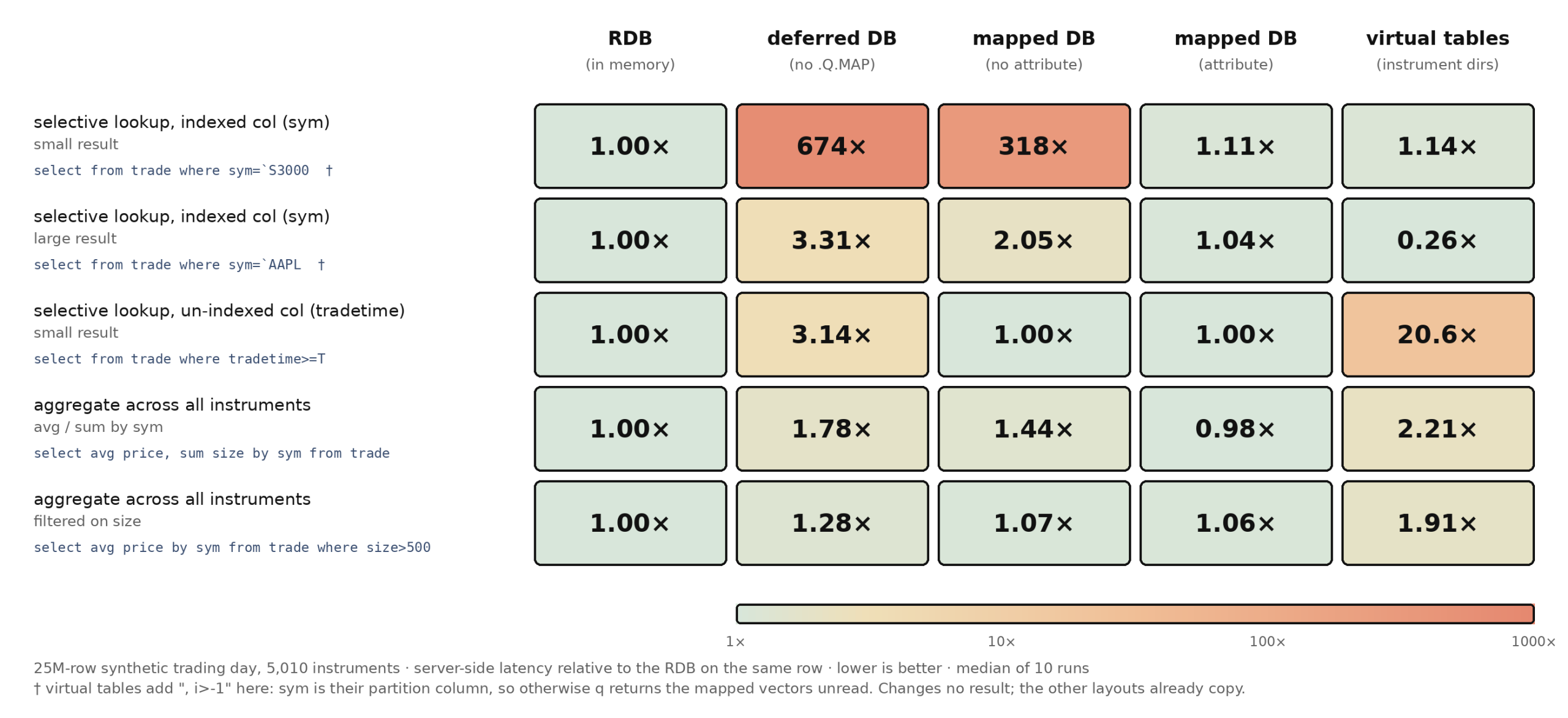
In the figure, RDB is standard TorQ, deferred DB is No-RDB with .Q.MAP turned off, mapped DB (no attribute) is No-RDB’s default, and mapped DB (attribute) is No-RDB with its new opt-in in-memory index. With 5,010 instruments, this dataset is close to a worst case for the virtual-table layout. This comes down to the cost of having to visit many directories for queries that do not specify an instrument.
When a query names an instrument, the directory effectively acts as the index. A small lookup comes in at 1.1× the RDB, while still being nearly 300× faster than the default No-RDB setup. The large lookup is 3.8× faster than the RDB because the result is already in one contiguous directory on disk, so the rows can be copied directly rather than gathered by index.
The same applies to historical days as well as the live day. Both the standard TorQ and No-RDB setups sort the day’s partition at end of day and apply a p#. The virtual-table layout never sorts, so it never gets a p# and never needs one. Every day has the same shape, which means every day answers the query in the same way.
However, the picture changes for queries that do not name an instrument. These have to visit every directory, and each directory adds a fixed amount of overhead regardless of how much data it contains. In this test, a time-range lookup was 21× slower than the RDB and even slower than No-RDB without .Q.MAP.
Queries that specify an instrument can go straight to a single directory. Queries that do not specify one, such as a lookup on tradetime or an aggregate, have to touch every directory. Their cost therefore grows with the number of instruments rather than just the number of rows.
Partitioning by instrument also means more directories and more small files, so the pressure shifts towards inodes and filesystem metadata rather than disk capacity. Backups are affected too, since the time they take depends more on the number of files than on the amount of data.
This means the setup is likely to work best where the instrument universe is reasonably fixed and not too large. FX is a good example, where the number of currency pairs is reasonably bounded. Instrument count matters for query performance as well as file count: a universe of 50 currency pairs and one of 5,000 equities will behave very differently. In markets where new instruments are added frequently, the number of directories and the cost of queries that have to visit them could grow quickly.
This layout isn’t intended to be a general-purpose replacement for every database design. The idea is simply to see what happens when the data is partitioned by instrument, and what we gain and lose by doing it this way.
Coming soon. Part two will look at what happens when the capture stack is split across multiple tickerplants, writers and intraday databases, all working against the same database.
Share this: