Conor Swain
KDB-X adds the ability for kdb+ to read Parquet files directly through its pq module, making it easier to fit kdb+ into wider data workflows. This blog explores what Parquet is and how it works within KDB-X, as well as demonstrating the development of a new pqx module tasked with extracting kdb+ data and saving it down in Parquet format, allowing for numerous customisation options. We will also look at the creation of virtual tables, which will allow for this Parquet data to be queried in the same way as you would query a kdb+ table that sits in an HDB on-disk.
Parquet in KDB-X
Apache Parquet is an open-source, column-oriented data file format designed for efficient data storage of large datasets. Data can be compressed using many different codecs like ZSTD and GZIP, which saves storage space while still allowing the files to be queried. This however comes at the cost of expensive reads into memory, as the Parquet data must be decoded in chunks before being worked with.
To help with this, KX have developed the pq module for KDB-X, which reads Parquet files directly into q. Individual files are mapped as virtual tables, and multiple files can be combined into a single larger virtual table that you query with standard qSQL. Row group and partition pruning keep the volume of data actually processed to a minimum. The practical benefit is interoperability: teams can exchange data with Spark, Pandas, Hive and Arrow without leaving KDB-X.
Before pq, the route into Parquet was arrowkdb, a long-standing Fusion interface that uses Apache Arrow as the intermediate format. Parquet is optimised for storage rather than computation, which is why it must be decoded in chunks. Arrow provides an uncompressed columnar layout that the CPU can work on directly once that decode has happened. The arrowkdb interface also writes kdb+ tables back out to Parquet, along with the Arrow IPC file and stream formats.
The pqx extraction module
The main task for this blog was to develop a new KDB-X module to enable both reads and writes of Parquet data. The module allows users to provide a set of customisation options around how data is saved down and packaged. The Parquet data on-disk can be queried directly using q-sql and operated on as if it were a kdb+ table.
Storage requirements for instruments can vary depending on liquidity. More liquid names could require tens of gigabytes, while the illiquid names may require mere kilobytes per day. Both extremities present issues. If a file is too large, the memory footprint required to manage it is significant and rewrites or corrections are expensive. The only way to improve performance comes from row grouping.
Memory overheads also present themselves when dealing with lots of smaller files – per-file footer reads and object-store GET and LIST costs make it extremely inefficient to store smaller instruments in single files.
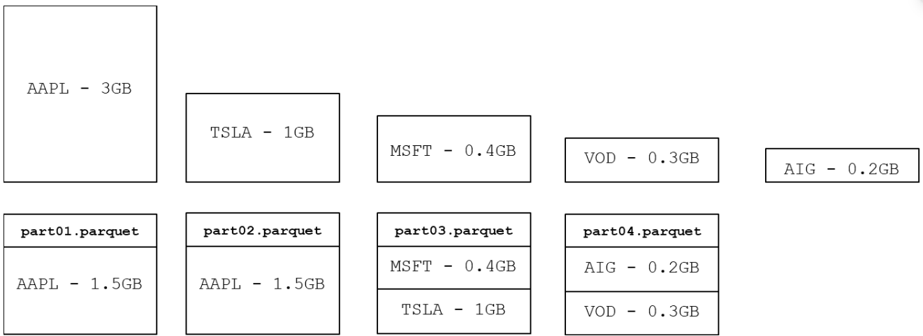
Options related to size, such as the size limit and the compression codec, can be customised in the module. By default, the writer is set up to generate files no larger than 1GB. This is implemented as a soft cap, which by default allows files to overshoot the target size by a factor of 1.5 – these sizes typically avoid the issues described above. When requested, the module will see larger instruments which exceed the size limit spread across multiple files, and package smaller instruments into one file until the size limit is met, then start a new file. The below diagram explains how large instruments are split into larger files, and smaller instruments are bucketed together.
Other options exist such as the ability to calibrate the compression ratio as part of the planning stage. With the provided codec, the module will perform a test write, and calibrate the ratio that is used to calculate how big an instrument is likely to be when persisted to disk.
As file writes are independent of each other and there is no issue with contention, it is also possible to parallelise writes of multiple files at the same time. Care should be taken when it comes to dictating how many threads are used, with memory being the primary consideration as opposed to core count.
Testing out the pqx module
There are several use cases that can be demonstrated with the pqx module. For this, we will be using data tables that have been created using the tickerplant setup provided in our Finance Starter Pack.
The main pqx extract function takes four parameters:
- kdb+ table of data
- table name
- date
- a dictionary of override options
Bucketing multiple syms per file
The first example demonstrates an extract call with size limits applied. For the purposes of this example, we are requesting a target size of 10MB, with an allowance of 20% on top of this. We have also provided the directory that this will be saved down to.
opts:(`targetsize`maxfactor`outdir!
  (10*1024*1024;1.2;`$(":/home/cswain/parquetHDB/")));

pqx.extract[tbl;
            `quote;
            2025.03.01;
            opts
            ]
The extract call returns a manifest of the contents of each file which can be seen below. Contents that are tracked include syms within the file and boundary values. Observe that multiple syms are packed within each file in this example. Note how IBM would have breached the size limit for file part-00003, hence a new file was commenced.
file                                                              seq virtualcols syms                    nsyms rows    mintime                       maxtime                       estbytes bytes    split status
------------------------------------------------------------------------------------------------------------------------------------------------------------------------------------------------------------------
:/home/cswain/parquetHDB/quote/date=2025.03.01/part-00001.parquet 1               `DOW`HPQ`INTC`GOOG`AAPL 5     1223297 2025.03.01D00:00:00.512764523 2025.03.01D23:59:59.901728364 11424523 11611658 0     ok
:/home/cswain/parquetHDB/quote/date=2025.03.01/part-00002.parquet 2               `AIG`MSFT               2     1009007 2025.03.01D00:00:00.198276402 2025.03.01D23:59:59.847182921 9423242  10162627 0     ok
:/home/cswain/parquetHDB/quote/date=2025.03.01/part-00003.parquet 3               `AMD`DELL               2     1188193 2025.03.01D00:00:00.172948578 2025.03.01D23:59:59.837261093 11096682 11193037 0     ok
:/home/cswain/parquetHDB/quote/date=2025.03.01/part-00004.parquet 4               ,`IBM                   1     684523  2025.03.01D00:00:00.964651809 2025.03.01D23:59:59.765009987 6392845  7916712  0     ok
Splitting the giants
Let’s say that for the next day, we want to enforce a 2MB limit on the file size, with the 20% allowance also included. Note how the larger instruments are spread across multiple files, while the smaller DOW and HPQ instruments have been able to be packaged in a single file. In the case that an instrument is spread across multiple files, the split flag returns true in the manifest.
opts:(`targetsize`maxfactor`outdir!
  (2*1024*1024;1.2;`$(":/home/cswain/parquetHDB/")));

pqx.extract[tbl;
            `quote;
            2025.03.02;
            opts
          ]
file                                                              seq virtualcols syms     nsyms rows   mintime                       maxtime                       estbytes bytes   split status
-------------------------------------------------------------------------------------------------------------------------------------------------------------------------------------------------
:/home/cswain/parquetHDB/quote/date=2025.03.02/part-00001.parquet 1               ,`INTC   1     144857 2025.03.02D00:00:00.289116795 2025.03.02D11:59:11.565188153 1346988  1895353 1     ok
:/home/cswain/parquetHDB/quote/date=2025.03.02/part-00002.parquet 2               ,`INTC   1     144856 2025.03.02D11:59:11.964961347 2025.03.02D23:59:59.165201611 1346988  1825710 1     ok
:/home/cswain/parquetHDB/quote/date=2025.03.02/part-00003.parquet 3               ,`GOOG   1     162053 2025.03.02D00:00:02.000000000 2025.03.02D12:01:31.165147994 1506890  1353027 1     ok
:/home/cswain/parquetHDB/quote/date=2025.03.02/part-00004.parquet 4               ,`GOOG   1     162052 2025.03.02D12:01:31.165147994 2025.03.02D23:59:59.165201611 1506890  1318508 1     ok
:/home/cswain/parquetHDB/quote/date=2025.03.02/part-00005.parquet 5               ,`AAPL   1     197801 2025.03.02D00:00:00.251728109 2025.03.02D12:02:33.564876824 1839303  1825986 1     ok
:/home/cswain/parquetHDB/quote/date=2025.03.02/part-00006.parquet 6               ,`AAPL   1     197800 2025.03.02D12:02:33.564876824 2025.03.02D23:59:59.354098762 1839303  1741075 1     ok
:/home/cswain/parquetHDB/quote/date=2025.03.02/part-00007.parquet 7               ,`AIG    1     234391 2025.03.02D00:00:00.182765301 2025.03.02D12:02:32.765318951 2179550  2785889 1     ok
:/home/cswain/parquetHDB/quote/date=2025.03.02/part-00008.parquet 8               ,`AIG    1     234391 2025.03.02D12:02:32.765318951 2025.03.02D23:59:59.640912673 2179550  2589710 1     ok
:/home/cswain/parquetHDB/quote/date=2025.03.02/part-00009.parquet 9               ,`MSFT   1     181058 2025.03.02D00:00:00.097261524 2025.03.02D08:02:01.965219087 1683612  1365472 1     ok
:/home/cswain/parquetHDB/quote/date=2025.03.02/part-00010.parquet 10              ,`MSFT   1     181058 2025.03.02D08:02:02.365320211 2025.03.02D15:59:51.364960436 1683612  1323413 1     ok
:/home/cswain/parquetHDB/quote/date=2025.03.02/part-00011.parquet 11              ,`MSFT   1     181056 2025.03.02D15:59:51.364960436 2025.03.02D23:59:59.765109271 1683612  1312246 1     ok
:/home/cswain/parquetHDB/quote/date=2025.03.02/part-00012.parquet 12              ,`AMD    1     192682 2025.03.02D00:00:00.122631524 2025.03.02D08:02:40.364904436 1791701  2459543 1     ok
:/home/cswain/parquetHDB/quote/date=2025.03.02/part-00013.parquet 13              ,`AMD    1     192682 2025.03.02D08:02:40.364904436 2025.03.02D16:01:13.565231754 1791701  2285573 1     ok
:/home/cswain/parquetHDB/quote/date=2025.03.02/part-00014.parquet 14              ,`AMD    1     192680 2025.03.02D16:01:13.565231754 2025.03.02D23:59:59.519200126 1791701  1969578 1     ok
:/home/cswain/parquetHDB/quote/date=2025.03.02/part-00015.parquet 15              ,`DELL   1     204678 2025.03.02D00:00:00.217354172 2025.03.02D07:59:56.364740856 1903249  1503707 1     ok
:/home/cswain/parquetHDB/quote/date=2025.03.02/part-00016.parquet 16              ,`DELL   1     204678 2025.03.02D07:59:56.364740856 2025.03.02D15:57:01.564615991 1903249  1511960 1     ok
:/home/cswain/parquetHDB/quote/date=2025.03.02/part-00017.parquet 17              ,`DELL   1     204676 2025.03.02D15:57:03.964602676 2025.03.02D23:59:59.965517225 1903249  1490254 1     ok
:/home/cswain/parquetHDB/quote/date=2025.03.02/part-00018.parquet 18              ,`IBM    1     228891 2025.03.02D00:00:00.023401288 2025.03.02D08:02:43.564593612 2128407  2903886 1     ok
:/home/cswain/parquetHDB/quote/date=2025.03.02/part-00019.parquet 19              ,`IBM    1     228891 2025.03.02D08:02:43.564593612 2025.03.02D15:59:55.364445853 2128407  2832644 1     ok
:/home/cswain/parquetHDB/quote/date=2025.03.02/part-00020.parquet 20              ,`IBM    1     228891 2025.03.02D15:59:55.364445853 2025.03.02D23:59:59.198201181 2128407  2936282 1     ok
:/home/cswain/parquetHDB/quote/date=2025.03.02/part-00021.parquet 21              `DOW`HPQ 2     216812 2025.03.02D00:00:00.081203974 2025.03.02D23:59:59.222812516 2016087  2005877 0     ok
Building custom plans
KDB-X gives us the ability to make functions public or private, which dictates whether they can be called ad hoc by the user. In the pqx module, several functions have been made public to allow users to test out various options to see how they affect instrument packing.
When extract is run with a one-shot call, it works by using “next-fit” packing, which will prevent a file from being added to as soon as an instrument is believed to breach the upper limit, even if smaller instruments come later which could fit that gap.
To test out the effect of different codecs, estimate can be run by providing the input partition data, the input options and Parquet write options. The latter two would need to be modified in this case, by providing an override for the codec value in the opts dictionary and the COMPRESSION value in writeopt. The expected file sizes can then be reviewed by taking the first item of the output of estimate. This example compares the difference between a codec of zstd and uncompressed.
first pqx.estimate[t;opts;writeopt]
sym  rowcnt estbyt
-------------------
DOW  36076  336829
HPQ  179827 1678982
INTC 288097 2689861
GOOG 324303 3027904
AAPL 394994 3687921
AIG  469004 4378927
MSFT 540003 5041819
AMD  576480 5382392
DELL 611713 5711351
IBM  684523 6391152
first pqx.estimate[t;
                  opts,(enlist[`codec]!enlist `uncompressed);
                  writeopt,(enlist[`COMPRESSION]!enlist `UNCOMPRESSED)]
sym  rowcnt estbyt
--------------------
DOW  36076  411423.7
HPQ  179827 2050812
INTC 288097 3285562
GOOG 324303 3698468
AAPL 394994 4504654
AIG  469004 5348691
MSFT 540003 6158389
AMD  576480 6574386
DELL 611713 6976196
IBM  684523 7806547
These outputs can then be used in the plan function to see how files are likely to be packed, as well as to test out different target sizes. For example, we can observe the difference that the new codec would make by using the new table of file sizes and passing it into plan. Note that the new uncompressed codec would require additional files for AIG and IBM compared to the zstd codec.
pqx.plan[symstats;opts;maxsize]
syms     seqno    estbytes
-----------------------------------------
,`INTC   1 2      1344931 1344931
,`GOOG   3 4      1513952 1513952
,`AAPL   5 6      1843961 1843961
,`AIG    7 8      2189463 2189463
,`MSFT   9 10 11  1680606 1680606 1680606
,`AMD    12 13 14 1794131 1794131 1794131
,`DELL   15 16 17 1903784 1903784 1903784
,`IBM    18 19 20 2130384 2130384 2130384
`DOW`HPQ ,21      ,2015811
pqx.plan[symstats_uncompressed;opts;maxsize]
syms     seqno       estbytes
----------------------------------------------------
,`INTC   1 2         1642781 1642781
,`GOOG   3 4         1849234 1849234
,`AAPL   5 6         2252327 2252327
,`AIG    7 8 9       1782897 1782897 1782897
,`MSFT   10 11 12    2052796 2052796 2052796
,`AMD    13 14 15    2191462 2191462 2191462
,`DELL   16 17 18    2325399 2325399 2325399
,`IBM    19 20 21 22 1951637 1951637 1951637 1951637
`DOW`HPQ ,23         ,2462236
To test different target sizes, we can overwrite the maxsize parameter and the targetsize option with new values. For example, if we want to plan for the uncompressed codec with a larger target file size like 5MB, we can see that fewer files are required.
pqx.plan[symstats_uncompressed;
        opts,(enlist[`targetsize]!enlist (5*1024*1024));
        (5*1024*1024)*opts[`maxfactor]]
syms          seqno estbytes
-----------------------------------
,`AMD         1 2   3287193 3287193
,`DELL        3 4   3488098 3488098
,`IBM         5 6   3903274 3903274
`DOW`HPQ`INTC ,7    ,5747798
,`GOOG        ,8    ,3698468
,`AAPL        ,9    ,4504654
,`AIG         ,10   ,5348691
,`MSFT        ,11   ,6158389
Hive partitioned database
The extract function can save down the table in a Hive-partitioned format in preparation for making use of virtual tables. “Hive” refers to Apache Hive’s partitioning convention, whereby instead of encoding a partition value only in a directory name, Hive partitions use key=value directory naming e.g. sym=AAPL, sym=MSFT. This can be repeated across multiple levels – in this example, we will request that the table be saved down by sym and src.
opts:(`virtualcols`outdir!
  (`sym`src;`$(":/home/cswain/parquetHDB/")));

pqx.extract[tbl;
            `quote;
            2025.03.03;
            opts
          ]
This means that there will be one file outputted for each sym from each src, creating the file structure below
/home/cswain/parquetHDB/quote
└── date=2025.03.03
    ├── manifest.json
    ├── sym=AAPL
    │   ├── src=BARX
    │   │   └── part-00001.parquet
    │   ├── src=DB
    │   │   └── part-00002.parquet
    │   ├── src=GETGO
    │   │   └── part-00003.parquet
    │   └── src=SUN
    │       └── part-00004.parquet
...
    └── sym=MSFT
        ├── src=BARX
        │   └── part-00037.parquet
        ├── src=DB
        │   └── part-00038.parquet
        ├── src=GETGO
        │   └── part-00039.parquet
        └── src=SUN
            └── part-00040.parquet
Parquet and Virtual Tables
The pq module gives users the ability to create virtual tables which can be queried in a similar way to partitioned tables in kdb+, which the pqx module has further wrapped to cast the virtual columns to their own types.
Let’s take the example of the Hive-partitioned database built above using the pqx extraction logic.
First we demonstrate a standard query on a similar kdb+ HDB table.
q)\l /home/cswain/hdb/
q)select from quote where date = 2025.03.04, sym=`AAPL, src=`GETGO
date       time                          sym  bid   ask   bsize asize mode ex src
-----------------------------------------------------------------------------------
2025.03.04 2025.03.04D00:00:00.602122826 AAPL 36.44 37.25 102   66    O    N GETGO
2025.03.04 2025.03.04D00:00:00.602122826 AAPL 36.09 37.23 109   102   Y    N GETGO
2025.03.04 2025.03.04D00:00:00.964666313 AAPL 36.43 37.76 19    94    H    N GETGO
2025.03.04 2025.03.04D00:00:01.364221900 AAPL 36.39 36.95 68    27    Y    N GETGO
2025.03.04 2025.03.04D00:00:03.365254281 AAPL 36.11 36.7  107   154        N GETGO
..
In kdb+ partitioned tables, data is not held in memory. Only certain metadata on the table is held in memory, such as the list of date partitions and column names. When a user queries a partitioned table (assuming the query is well-formed), the OS will first access what partitions the query is interested in. The example above is set up as a date-partitioned database, so the q-sql query will only access the 2025.03.04 partition. From there, the columns that are being queried on are read in to compare against the constraints, before the result set is returned to the user.
With the KDB-X Parquet module, virtual tables are set up in a similar way. A function called mkP exists within the pq.t sub-module which allows for the creation of virtual tables – this pq.t module will need to be loaded in separately, though the pqx module takes care of that at initialisation.
mkP works by creating partitioned virtual tables from a key table comprised of the partition values and a list of virtual Parquet tables. In our example, the partition values would be date, sym and src. The virtual Parquet tables are simply made up of the return of pq.pq[path], which turns a Parquet file into a virtual table. That table is then attached to the key columns.
In the pqx module, we wrap this within the buildvirtualtable function to bring all of the files together. All that is required is the HDB directory of the Parquet files, the table name and a dictionary mapping of the virtual columns and their types (in the order that they sit on disk).
The virtual tables can then be queried in the same way as you would query a kdb+ partitioned table. A well-formed query will reduce the number of files that are accessed to get your results set, so ensure your virtual columns are the first columns to be queried in your where clause.
q)quote:pqx.buildvirtualtable[`$":/home/cswain/testParquet";`quote;`date`sym`src!"DSS"]
q)select from quote where date = 2025.03.04, sym=`AAPL, src=`GETGO
date       sym  src   time                          bid   ask   bsize asize mode ex
-------------------------------------------------------------------------------------
2025.03.04 AAPL GETGO 2025.03.04D00:00:00.602122826 36.44 37.25 102   66    ,"O" ,"N"
2025.03.04 AAPL GETGO 2025.03.04D00:00:00.602122826 36.09 37.23 109   102   ,"Y" ,"N"
2025.03.04 AAPL GETGO 2025.03.04D00:00:00.964666313 36.43 37.76 19    94    ,"H" ,"N"
2025.03.04 AAPL GETGO 2025.03.04D00:00:01.364221900 36.39 36.95 68    27    ,"Y" ,"N"
2025.03.04 AAPL GETGO 2025.03.04D00:00:03.365254281 36.11 36.7  107   154   ," " ,"N"
..
Limitations and Future Work
While the pqx module can cope with a wide range of use cases, there are a number of paths that can be explored in future development.
Next-fit packing
As mentioned previously, the current packing mechanism will prevent a file from being added to as soon as an instrument is believed to breach the upper limit. Consult the diagram at the beginning of the article. An instrument of size 50MB could fit in part03 alongside MSFT and TSLA, but because an earlier instrument did not fit, that bucket is closed. A change to what is known as “first-fit packing” could mitigate this by checking all buckets and adding the instrument to the first bucket that it fits in.
Non-uniform compression
Compression is not uniform through the writedown process, even though the codec remains the same for each file write. The ratio can vary over the course of the run, and it is possible that files may end up larger or smaller than was planned. There could be checks implemented after each file write to review the compression ratio and re-run the plan accordingly if a discrepancy in the ratio is encountered, which could ensure most efficient packing.
One file per virtual table partition
Currently the building of virtual tables is limited to one file per virtual partition, meaning it would be a challenge to incorporate the likes of the split larger instruments into the virtual table construction. One work-around of this could be to use the manifest to bring the multiple files together within one partition on the face of it, even if the paradigm of one file per partition would still hold true under the hood.
Conclusion
Together, the pqx module and virtual tables let KDB-X users extract kdb+ data into Parquet files sized to each instrument’s liquidity, then query that data with the same partition-aware syntax used against an on-disk HDB. Parquet’s storage efficiency and interoperability with tools like Spark and Pandas come without changing how the data is queried. The result is a workflow that stays entirely within KDB-X, from extraction through to querying, without handing data off to another system.
Useful Links
KX’s arrowkdb interface can be found here, and can be downloaded through their Anaconda channel. Further documentation can be found in the repo.
The pqx module forms part of DI’s KDB-X GitHub, which can be found here. Documentation on how to use these modules can also be found through the same link.
The “Finance Starter Pack” that was used to build the kdb+ database can be found here. This implements the TorQ framework to provide a working example of a production-ready market data capture system.
Share this: