When is a Feed Handler Fast Enough?

Germans Zaharovs

When does low latency matter?

Within software development, low latency refers to the ability to provide a response to an input with minimum delay. It is prevalent in industries and applications such as video gaming, real time embedded systems, and High Frequency Trading. These are the leading domains that require speed, otherwise software would simply be unusable. High Frequency Trading (HFT) is considered to be one of the most performance-critical software environments, due to the competitive nature of the financial markets. Every nanosecond matters!

Usual software development practices such as an object oriented development approach or standard design patterns may not produce the fastest code in practice. Features such as Single Instruction Multiple Data (SIMD), branch predictions and manipulation of CPU cache (keeping caches hot) play their role in low latency.

There is a long list of things to consider during low latency application development. Some common advice when measuring the performance of software:

Don’t assume things – run it and check the performance. If code has not been performance measured, all assumptions will be just assumptions.
Pay much more attention to the biggest bottlenecks of the code instead of over-optimizing parts that are seldom used.
Don’t assume, that ordinary software development practices would produce the best performance results (e.g. Big O notation). More needs to be considered – SIMD, cache friendliness, contiguous memory, keeping hot path hot, etc.

The best advice is to experiment and measure differences.

So how do we achieve all of the above? How do we measure that a feed handler is fast enough?

One convenient tool, which this blog will focus on, is ‘valgrind’. Specifically the ‘callgrind’ tool, which focuses on profiling CPU/cache performance. It is a well-known tool in the profiling industry and I believe it brings unique capabilities to make performance testing easier, well-presented, and more accurate.

Here is an intro to ‘valgrind’, which you likely will find useful. It contains lots of information about the tool. Whilst the intro/reference materials are very well presented, they are comprehensive and require time to read/experiment and understand intentions. Providing an example of how valgrind can be used is a good introduction for many to start using valgrind/callgrind to profile software.

One of the latest projects I have been working on required building a Limit Order Book (LOB). This could be a good example of how profiling tools may be used to improve performance. The first implementation of LOB used std::set (red/black self-balanced tree, or simply rbtree). This approach possesses features of worst case complexity O(log n) whilst on average it is almost O(1) for insertions & deletions. Even though some resources suggest that rbtree doesn’t provide the most optimized LOB implementation, at the time it was decided to go with rbtree because of the following:

Easy to implement.
Easy to prove concepts. It will be easier to reason, why rbtree is either slower, or faster when other approaches are to be implemented.
A deep understanding the purpose of more complex structures is required.

Valgrind

This blog isn’t solely about LOB, but performance, therefore lets focus on how valgrind/callgrind might be helpful to identify performance issues within the code.

To use valgrind effectively code should be compiled in ‘debug’ mode (which includes additional debug symbols). In GCC it could be achieved by providing a ‘-g’ flag during compilation, or ‘-DCMAKE_BUILD_TYPE=Debug’ in cmake projects. It is not actually a necessity for valgrind as it works by emulating CPU, but debug symbols provide additional information for users to easily identify bottlenecks within source code.

Valgrind significantly slows down the execution of software. Running a whole day market data canned file is unlikely to provide any more information than a subset of that file, which will execute much faster. Therefore only a subset of the canned file has been used for the test below.

valgrind –tool=callgrind <binary file> <arguments>

After executing above command, valgrind automatically starts <binary file> command and runs as a normal executable. During start valgrind provides info similar to below:

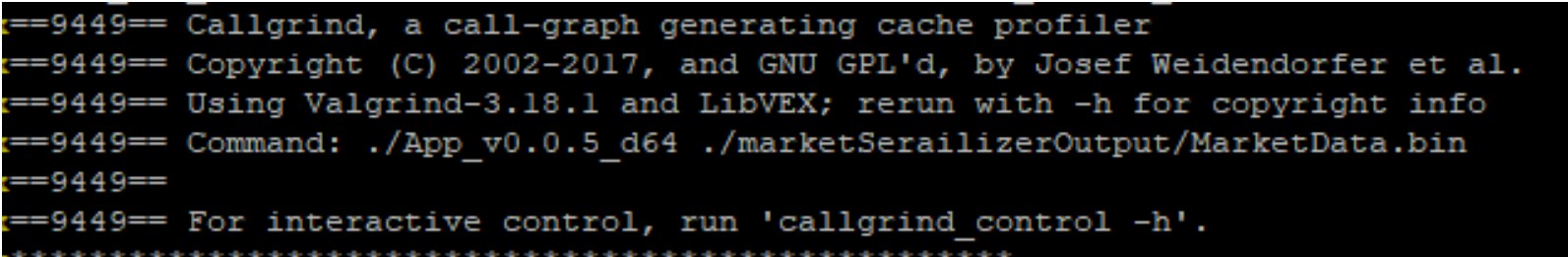
Here we can see Process ID (9449), valgrind version (3.18.1), tool being used (Callgrind), and command being executed (./App_v0.0.5_d64 ./marketSerailizerOutput/MarketData.bin).

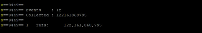
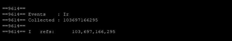
After the program finishes valgrind execution user will be notified of total number of CPU instructions (Ir – Instructions Read) being used by the program:

Callgrind/KCacheGrind

Even though it is perfectly possible to examine callgrind file on its own, or use some CLI tools (e.g. callgrind_annotate), ‘KcacheGrind’ GUI tool is useful to visualise callgrind output provided by valgrind.

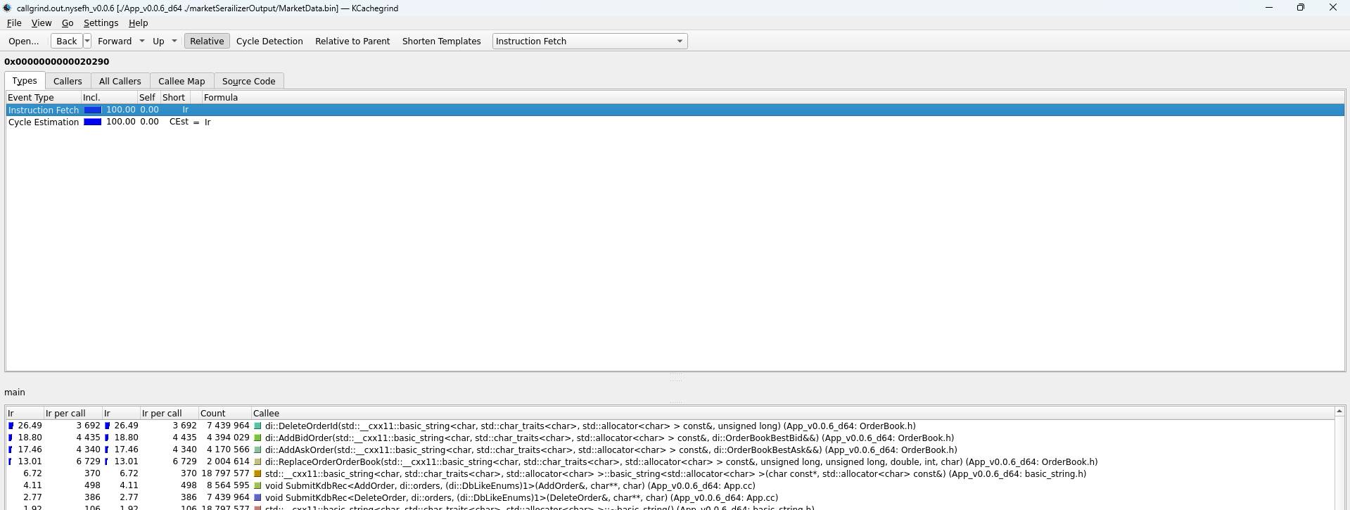
Understanding callgrind output (KCachegrind):

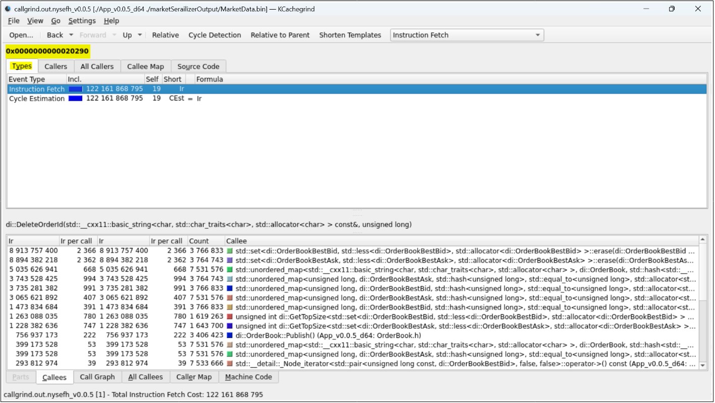
Above we can see that KCachegrind provides a lot of useful information. At the top, we can see that the ‘Types’ tab is selected and it sets the base memory address of the program (0x0000000000020290). ‘Instruction Fetch’ replicates a total number of CPU instructions output of valgrind mentioned earlier. ‘Cycle estimation’ can be used to calculate the approximate time being used, which is irrelevant at this moment.

The below tab ‘Callees’ provides highly valuable information – how many instruction cycles were used by the specific function of the program. By default, it is sorted by ‘Total Instructions Read’, which means most expensive calls. As we can see – the most expensive calls are for std::set<…>::erase. This makes it worth investigating. Specifically, it means to examine source code, to find if anything could be done to make it run more efficiently.

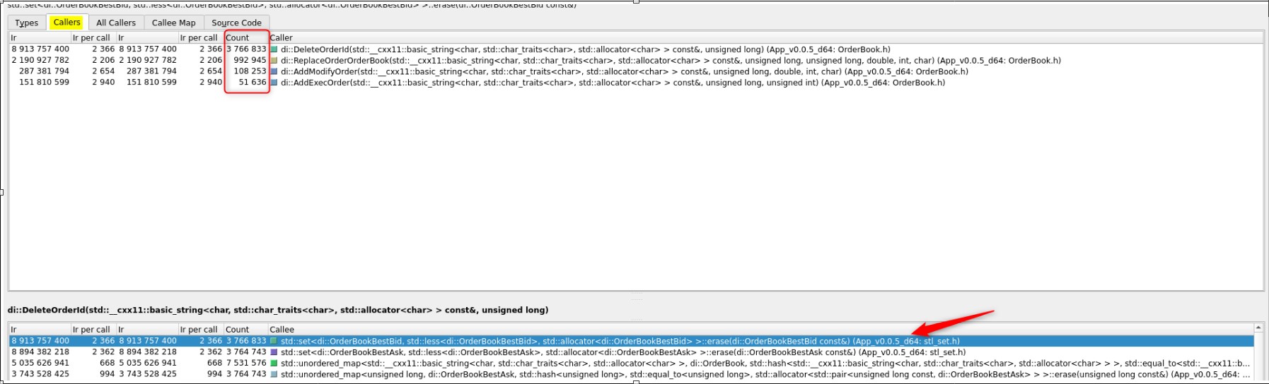
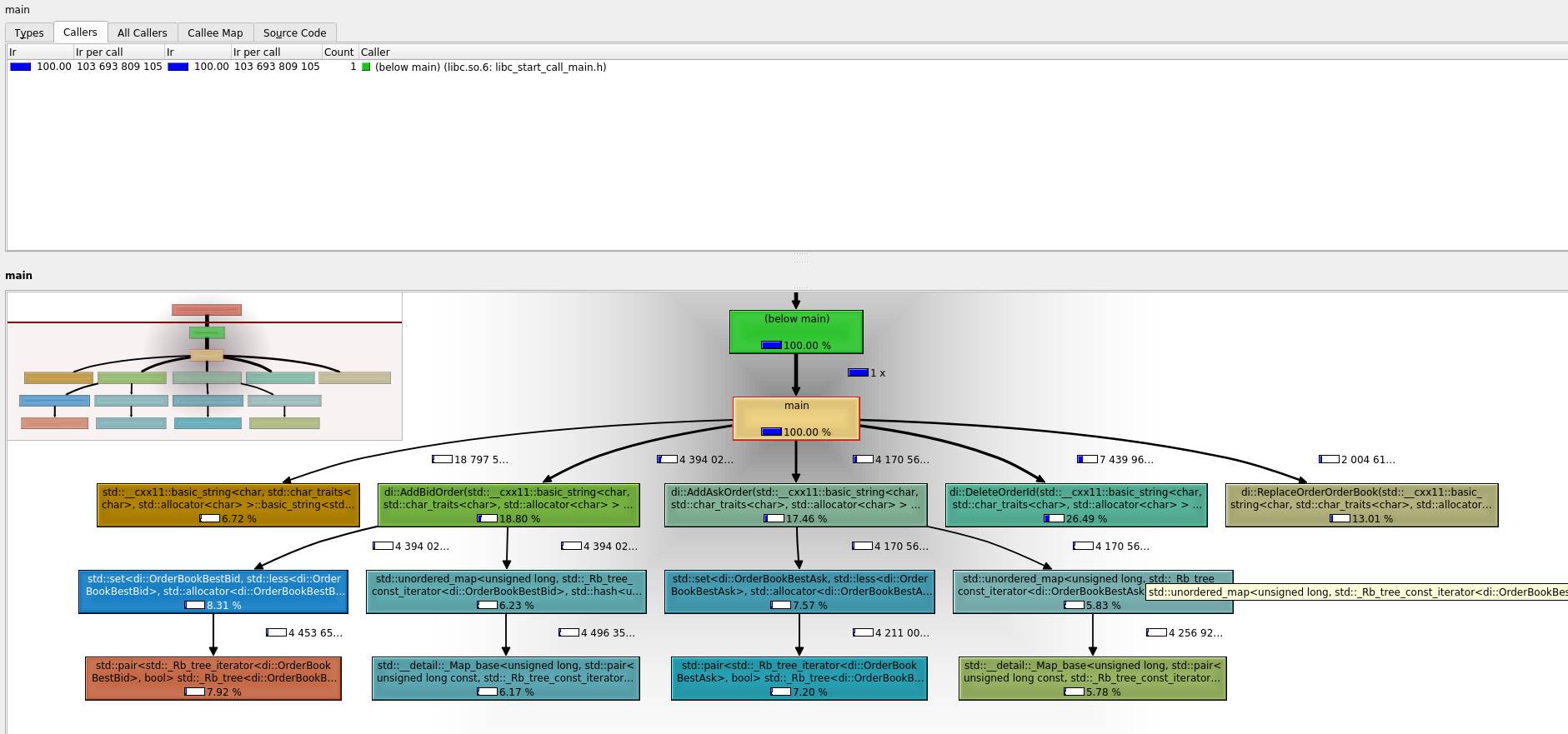
‘Callers’ tab (at the top) helps to see Instructions Read (Ir) executed per required function (std::set<…>::erase):

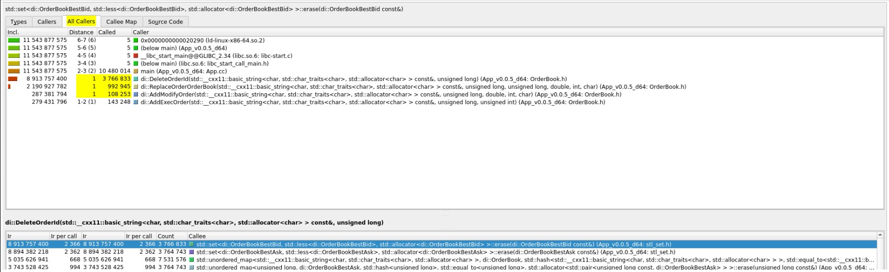
Quite similar functionality is provided by the ‘All Callers’ tab, which gives a hierarchy view of functions calling ‘std::set<…>::erase’:

‘Callee Map’ provides map visualisation of expensive call:

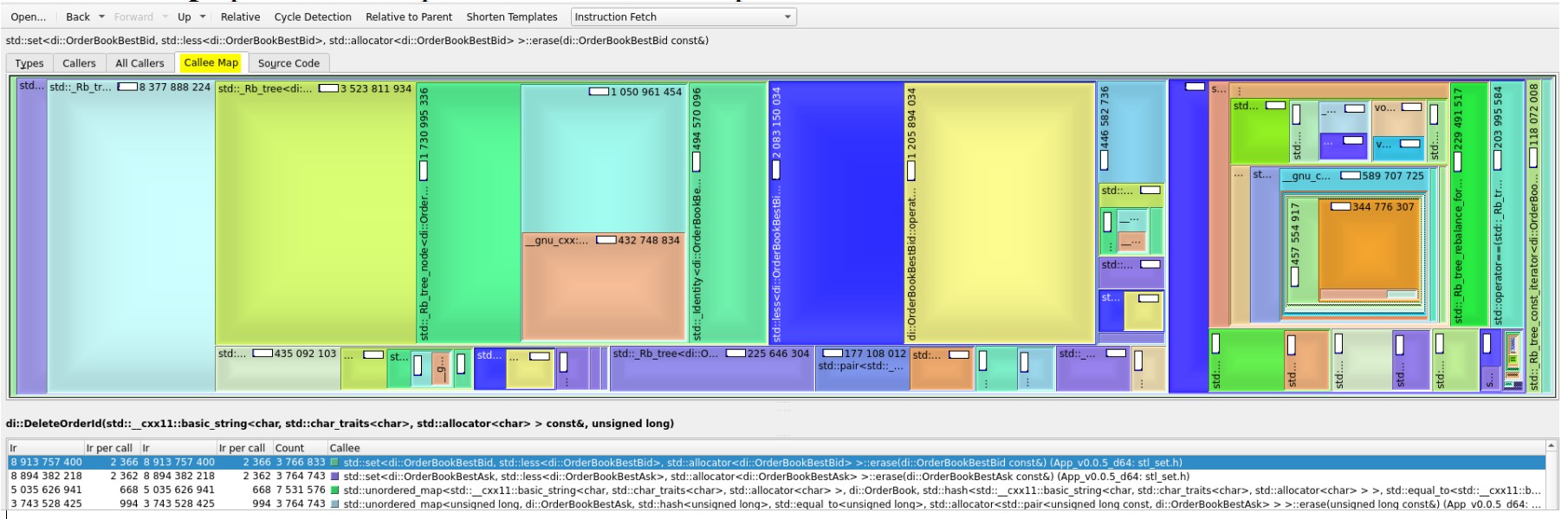
Above it is shown all parts of code, which makes this given call expensive. It might be useful for insight info.

Also, personally, I find ‘Callee Map’ (upper menu) and ‘Call Graph’ (bottom menu) useful to pinpoint expensive calls overall in software. This can be done by going to the very top of the software memory address (0x0000000000020290 address provided earlier):

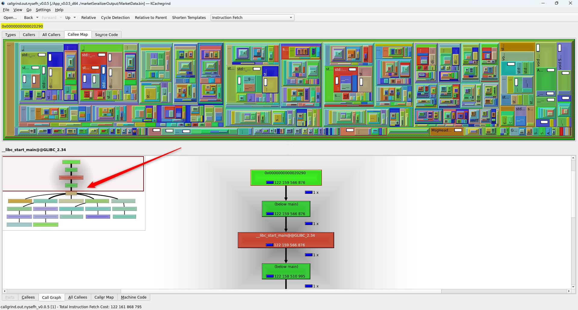
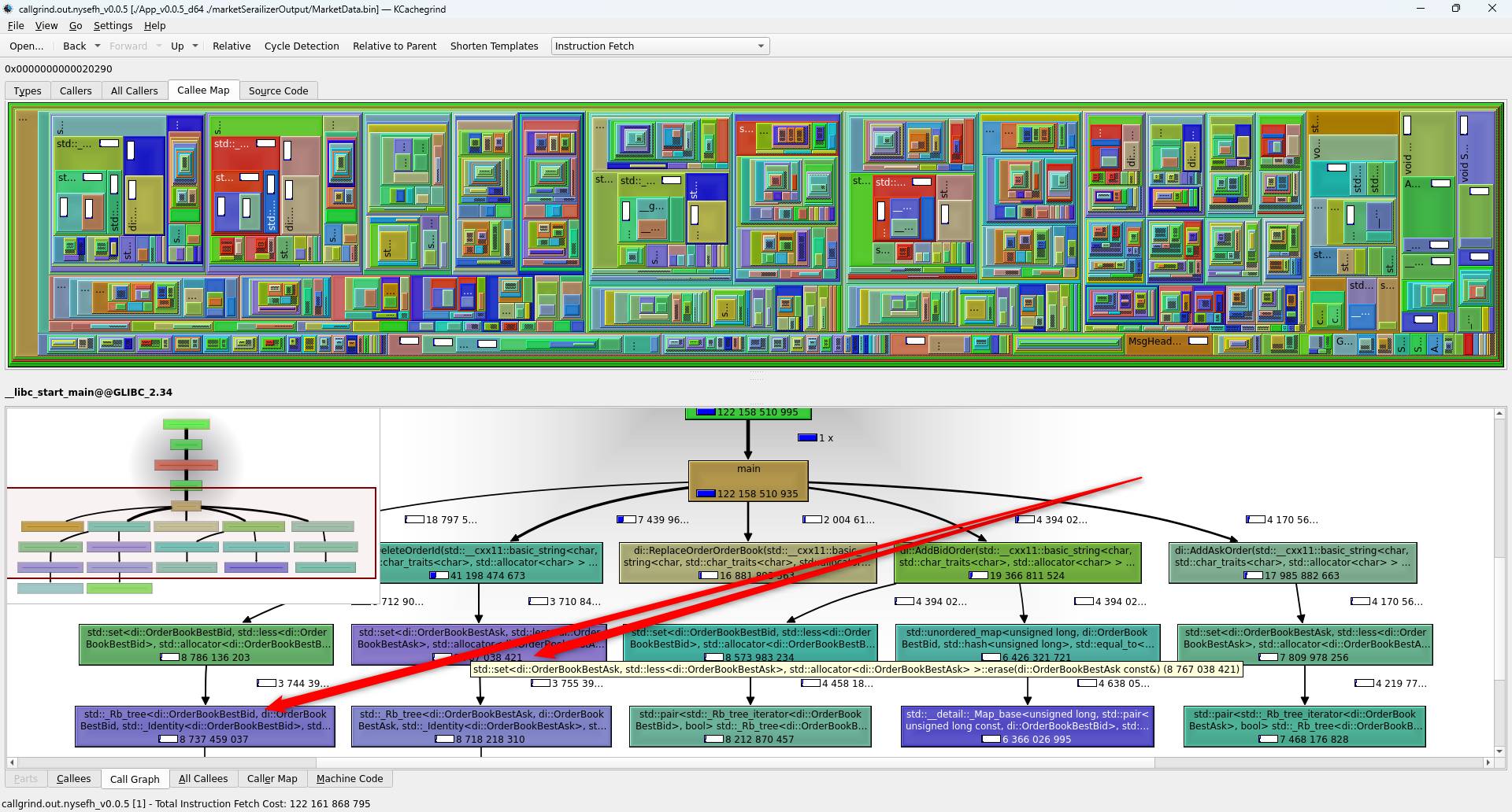
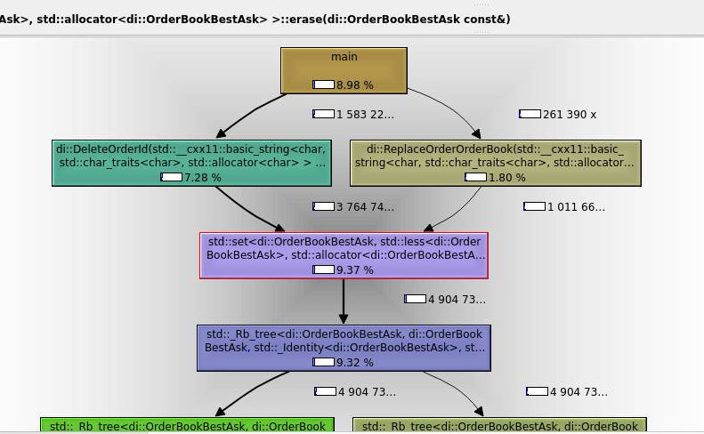
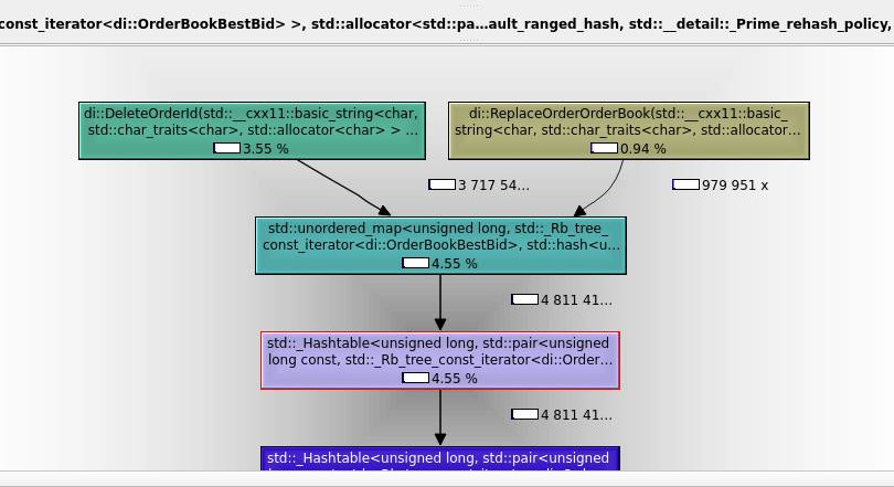
As we can see from above, it is easier to use ‘Call Graph’ to navigate to expensive ‘std::set<…>::erase’ function to be investigated:

Also ‘Relative’ option provides the overall percentage used per expensive call:

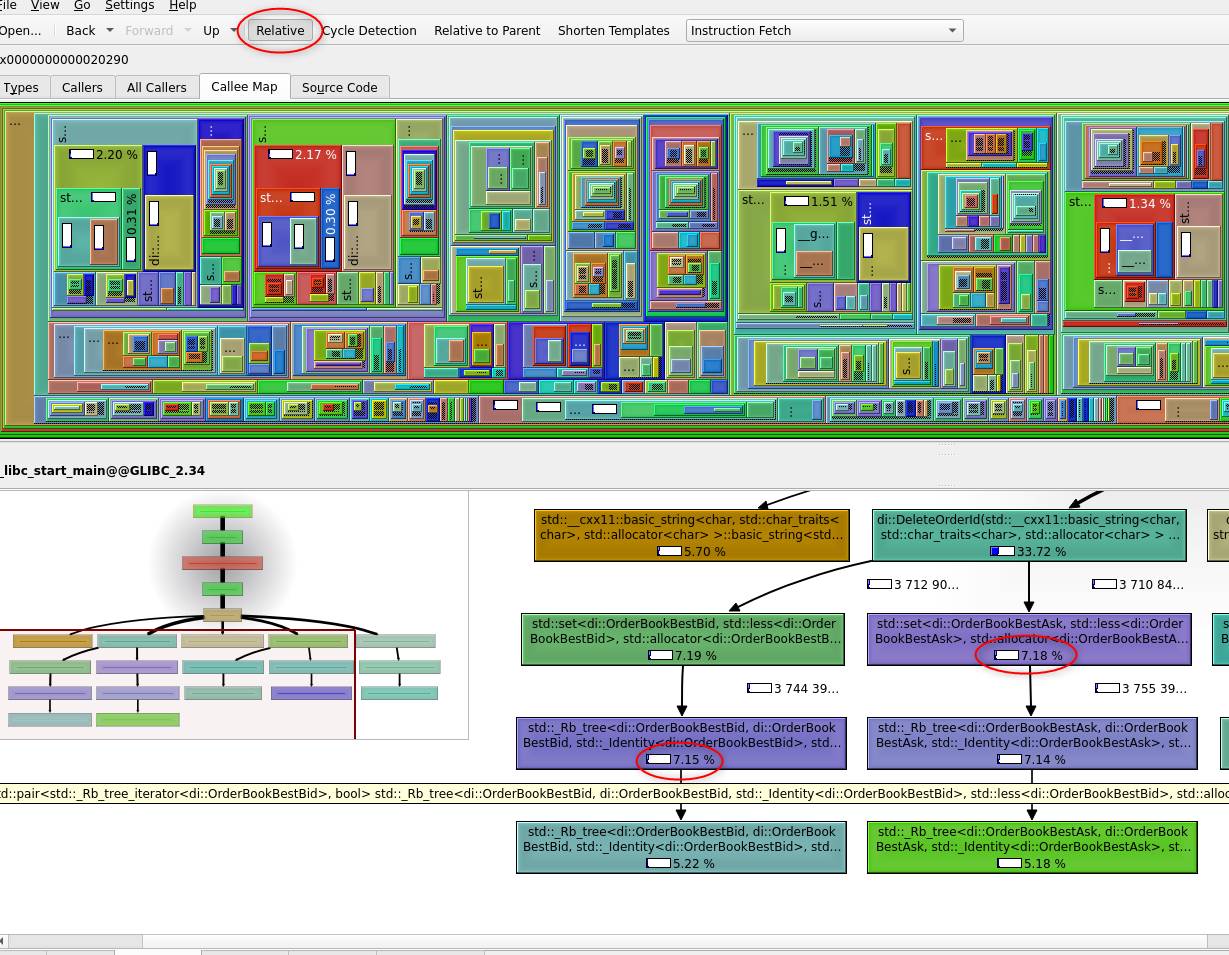
All of the above findings makes ‘std::set<…>::erase’ usage a strong candidate for investigation.

Source code investigation/modifications

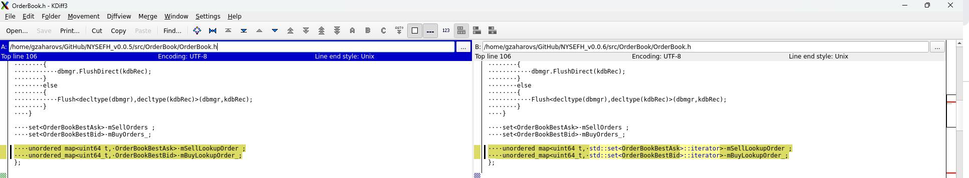
Looking at the code we can see, that rbtree sell and buy STL set containers are using lookups as unordered_map:

    set<OrderBookBestAsk> mSellOrders_;
    set<OrderBookBestBid> mBuyOrders_;

    unordered_map<uint64_t, OrderBookBestAsk> mSellLookupOrder_;
    unordered_map<uint64_t, OrderBookBestBid> mBuyLookupOrder_;

Each delete and creation of it currently is making an additional copy of the object:

pOrdBook->mSellOrders_.insert(askOrd);
pOrdBook->mSellLookupOrder_[askOrd.mOrderId_] = askOrd;

orderBookRefVal.mSellOrders_.erase(foundSell->second);
orderBookRefVal.mSellLookupOrder_.erase(orderId);

After reviewing C++ std::set API and knowing the expense of additional copy, it became clear, that using a single object, which is part of ‘std::set’ and using an iterator to this object as a lookup reference should be a lot cheaper.

Snap of changes implemented

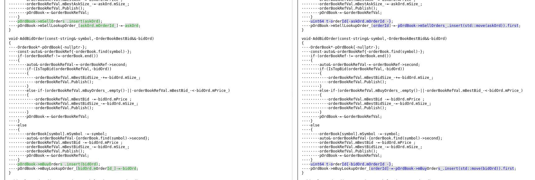
NOTE: Not only ‘std::set<…>::erase()’ would benefit from the above change, but also all associated lookup procedures, e.g. ‘find’, ‘update’, ‘insert’. This is due to the fact that the iterator strongly belongs to the std::set container which represents the required rbtree, and the iterator is cheaper in size. Logically the iterator is more strongly associated with the lookup map, than a copy of the object.

Running valgrind callgrind of updated code:

Immediately after run we can see, that Instruction Reads has far fewer number:

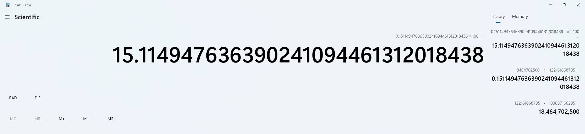
Making rough, quick calculations we can see, that code is about 15% faster after implementing the change:

Checking KCachegrind map/graph outputs to verify assumptions:

As we can see, now most expensive functions per application have been changed.

The above diagram suggests, that std::set<…>::erase is not part of the most expensive calls of the software anymore. Program runs faster by about 15% after this single improvement.

NYSEFH v0.0.5	NYSEFH v0.0.6

Conclusion

Profiling is a continuous process of improvement. It takes effort to review profiled data as well as review code that produces given data. This change was straightforward – eliminating unnecessary lookups and copies. Changes required to improve code might, or might not be straightforward. As an example, expensive calls might be due to specific third-party library calls, which software has no control of.

Valgrind allows us to visualise the biggest resource consumers in a short time and easily review these along the code. By examining and improving the biggest resource consumers we make the feed handler faster and more reliable in handling data. As demonstrated by the example, valgrind helped to identify an issue within LOB and improve the performance of the feed handler by about 15%.