TimescaleDB

TimescaleDB is a relational database system built as an extension on top of PostgreSQL.  This means it maintains full compatibility with PostgreSQL while incorporating additional features that enhance its optimisation for working specifically with time series data. Some of these features include:

• Automatic time-based partitions (called chunks)

• Built-in time-series specific functions

• Improved compression capabilities

• Continuous aggregates

These features are only enabled on TimescaleDB hypertables, which otherwise look and behave exactly like a regular PostgreSQL table. A hypertable can be created from either scratch or by converting a regular PostgreSQL table.

In this blog we will aim to give an introduction to some of these features of timescale and measure their impact on performance compared to a traditional PostgreSQL database.

Query Performance

Timescale enhances query performance for time series data primarily by utilising time-based partitions. Tables are divided into chunks that are categorised based on time periods. When a query is executed, Timescale first identifies the appropriate chunk instead of searching through the entire database. These partitions can also help with insert rates and compression which we will look at later.

By default, chunks are set to a period of 1 week. However, it is crucial to choose a chunk size that is optimized for your specific data and hardware. The official recommendation suggests that the chunk size should be around 25% of the available memory or roughly 1-20 million records. It is also important to note that once data has been inserted, the chunk sizes cannot be modified. Therefore, it is essential to establish the best chunk size during the initial creation of a hypertable.

To test query performance we have used a TimescaleDB database and PostgreSQL database which both contain two identical tables. First a trade table containing over 13 million records with 8 different metrics:

And a quote table which contains over 63 million records with 9 different metrics:

Both tables hold data spanning a 4-day duration. In the case of TimescaleDB hypertables, they are partitioned into 15 chunks, each covering a 6-hour period. The chunks for these tables will therefore contain approximately 4 million and 1 million records each.

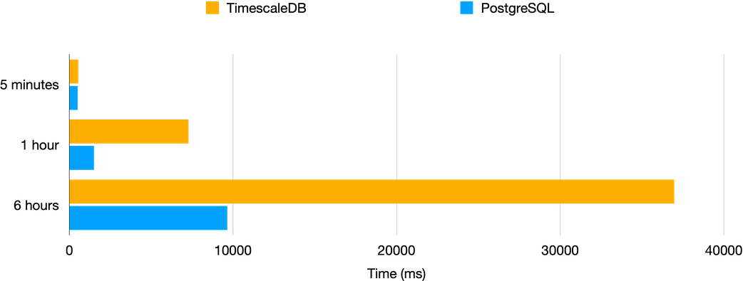
We start testing with a simple query, selecting 5 minutes of data from the quote table for a particular symbol:

After conducting several similar queries with varying times and symbols, and excluding the initial runs to account for caching effects, the average results obtained were as follows:

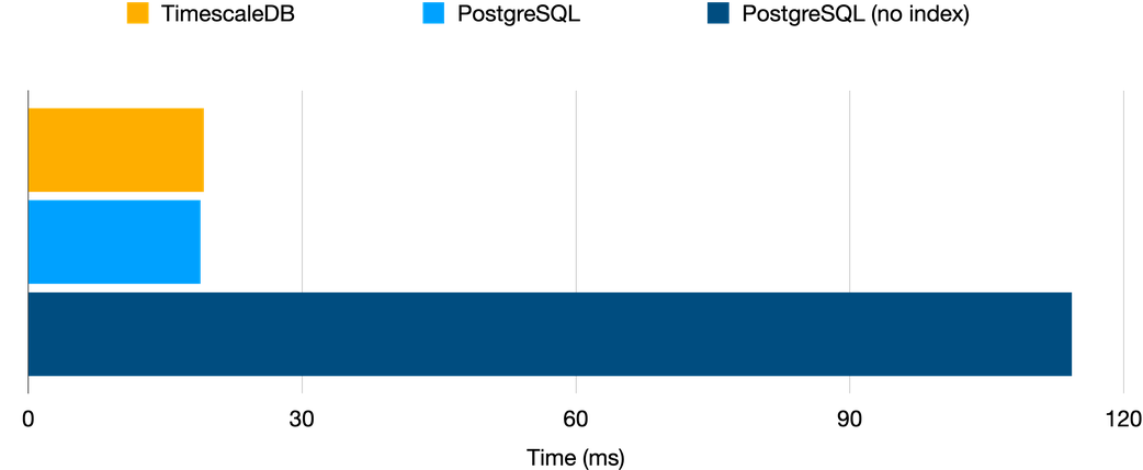
Despite the implementation of time-based partitions in TimescaleDB, it does not appear to provide significant improvements in this particular scenario. A significant portion of the performance gains seem to be derived from indexing, which is also available in PostgreSQL.

When performing these simple queries, TimescaleDB typically exhibits a slight increase in execution time compared to PostgreSQL. This additional time is attributed to the extra planning involved in locating the correct chunk. However, the advantage of TimescaleDB’s approach becomes more apparent when dealing with more complex queries. For instance, when testing a slightly more complex query that searches for the minimum ask and maximum bid within a 5-minute interval for each symbol, TimescaleDB demonstrates its effectiveness.

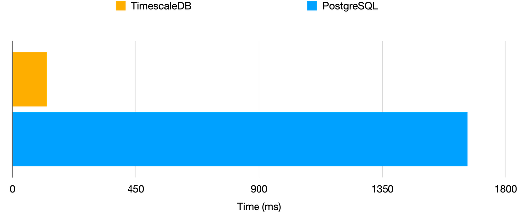
In this scenario, Timescale demonstrates significantly improved performance, aligning with my findings across many similar query types. It exhibits speeds up to 15 times faster compared to regular PostgreSQL.

An additional commonly used query for this type of market data is an as-of join. Neither PostgreSQL nor TimescaleDB have built-in capabilities for as-of joins; however, they can be accomplished manually. I conducted tests for various time periods, aiming to identify the prevailing bid and ask at the time of each trade using the following method:

This gave the following results:

In the case of performing the join over a 5-minute data interval, Timescale exhibits slightly inferior performance. However, as the duration increases, Timescale’s performance surprisingly becomes even worse compared to Postgres. It is worth noting that this as-of join method is likely far from the most efficient approach, and Timescale is actively prioritising the development of a built-in as-of join function that is should give better performance.

Hyperfunctions

While Timescale currently lacks a built-in as-of join capability, it offers numerous other built-in “hyperfunctions” that streamline data analysis. These functions are specifically optimized for time-series data and leverage the advanced features of Timescale’s hypertables.

One particularly useful function is time_weight which makes it very easy to compute time weighted averages. For example, the time weighted average spread over some period of time for each symbol will be given by:

The LOCF option (last observation carried forward) assumes that the spread remains constant until a new observation becomes available. On the other hand, the alternative option, LINEAR, assumes that values progress linearly from one observation to the next.

This code is significantly simpler compared to what would be necessary using regular SQL. Moreover, it enables the construction of more complex queries by building upon each other. For instance, we can combine this query with another hyperfunction called time_bucket. By leveraging this function, we can easily create time buckets to facilitate grouping operations.

This will give us the TWAS for each symbol across every 5 minute bucket within in quote table. TimescaleDB offers a vast array of over 100 hyperfunctions that can be utilised for various data analysis tasks. A comprehensive list of these hyperfunctions can be found here.

Continuous Aggregates

Continuous aggregates are a powerful feature of Timescale that simplify and accelerate data analysis by enabling the precomputation and storage of aggregated results on hypertables. This leads to a significant improvement in query performance for common analytical queries, as the results are precomputed and cached.

The functionality of continuous aggregates is similar to materialized views, a feature found in regular Postgres. The outcome of a query is stored as a physical object in the database, allowing it to be queried like a regular table to retrieve the results. However, materialized views encounter two challenges when working with real-time data:

1. Lack of automatic refresh: Views need to be manually refreshed to incorporate the latest available data.
2. Recalculation on the entire dataset: When refreshing to include new data, the same calculations are repeated on older data, resulting in redundant computations for time series data.

In contrast, continuous aggregates in Timescale require the creation of a refresh policy. This policy allows you to specify the frequency of aggregate refreshes and the time interval for recalculating the results. As an illustrative example:

This code snippet will generate a view that calculates and stores the high, low, open, and close values for each symbol within 5-minute time buckets. The defined policy ensures that the view is refreshed every 5 minutes, recalculating results only for data that is between 5 and 10 minutes old. This approach proves particularly valuable when we anticipate that only recent data will be inserted into the database, while older data remains unchanged.

It is possible to construct continuous aggregates based on other continuous aggregates, allowing us to summarise data at different levels of granularity. The process involves selecting from the previously created view instead of the original table when creating a new continuous aggregate. For instance, we could introduce an additional continuous aggregate that captures hourly high, low, open, and close (HLOC) data derived from the 5-minute HLOC data. This approach is considerably more efficient than utilising the original table once again. However, it is important to note that when working with hierarchical aggregates, the time interval of one aggregate must evenly divide into the time interval of the aggregate above it.

Insert Performance

Timescale improves insert performance by utilizing chunks that are ideally sized to fit into memory, thereby minimizing the requirement to swap pages from disk. In Postgres, the process of swapping pages from disk during large inserts can considerably slow down the insertion speed. By eliminating the need for this disk swapping, Timescale should significantly improve the rate at which inserts can be performed.

When it comes to inserting data that is small enough to fit within available memory, the performance improvement over regular PostgreSQL is not significant since the underlying process remains mostly unchanged. To evaluate this, I conducted tests where I inserted batches of 10,000 up to 1 million rows at a time using the execute_values function from the psycopg2 library in Python. This function enables bulk insertion of data from python into a Postgres database.

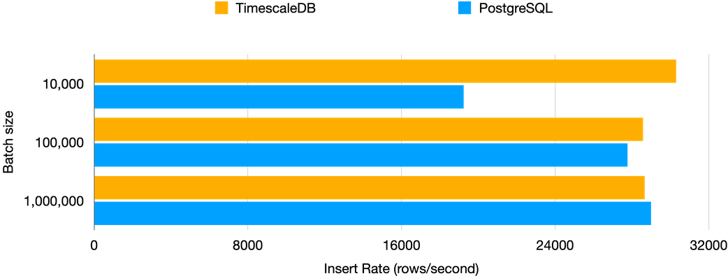
Given the small size of the data that can easily fit into memory, the disparity in the insert rate is negligible. To assess performance on a larger data scale, I conducted a test by bulk inserting the entire database, consisting of approximately 76 million rows, utilising the highly efficient COPY command in PostgreSQL, specifically designed for bulk inserts.

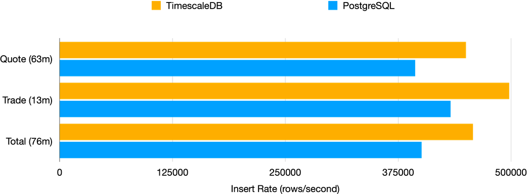
Although Timescale does give better performance, the difference in insert rates compared to PostgreSQL is only slightly over 10%. To truly see the advantages of Timescale’s insert performance, you would need to handle insertions on a much larger scale, involving hundreds of millions or even billions of rows.

Compression

Compression is a crucial aspect of Timescale, and its implementation differs significantly from regular Postgres compression. While Timescale still uses compression algorithms to minimise the disk space occupied by compressed data, it also goes beyond that by modifying the data layout on disk. This alteration can prevent slower queries on compressed data and, in certain instances, even lead to faster query performance on compressed data. Therefore, Timescale’s approach to compression not only reduces storage requirements but also optimises query execution on compressed data.

Timescale achieves this by consolidating segments of up to 1000 rows into a single row of data. In this transformed row, each column stores an ordered set of data that encompasses the entire column from the original 1000 rows. This restructuring effectively converts the table from a row-based storage format to a columnar storage layout, which offers improved efficiency for queries that target specific columns. This blog explains the compression process in full detail.

During the data compression process, it is possible to specify a field to order by and segment by. These choices have a significant impact on performance since compressing the data results in the removal of indexes (these will be automatically added back if uncompressed). Applying ‘segment by’ to the sym column will group symbols within each compressed row, and applying ‘order by’ to the time column will sort by time within each of these compressed rows.

Compression in Timescale operates on a per-chunk basis, meaning that compression is applied to entire chunks, and each original chunk corresponds to one compressed chunk. To automate the compression process for older chunks, you can configure a compression policy. It is advisable to leave the most recent chunk uncompressed since inserting data into compressed chunks is much slower.

You will also want to consider the number of records per sym (or whichever field you are segmenting by), per chunk, anything much less than 1000 and the table won’t be able to compress as efficiently. In our case we have roughly 10,000 so would expect roughly 10 compressed lines for each symbol per chunk.

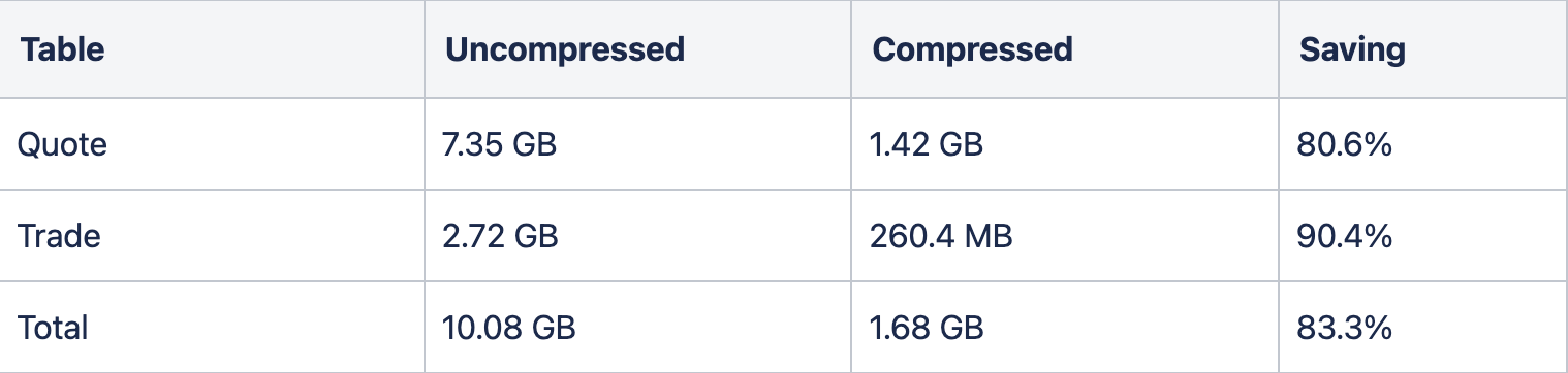
The overall compression achieved for our entire database is shown below, with a total compression rate of slightly over 83%. It is worth noting that the compression ratio will vary depending on the specific data, but columns with repetitive values or following certain patterns generally compress better than randomly distributed data.

When considering query performance, the impact of compression can vary depending on the specific queries being executed. The effectiveness of compression will be influenced by your dataset and the nature of the query itself. In general, you can anticipate that wider, shallower queries (focused on many columns over recent time periods) will perform better on uncompressed data. On the other hand, narrower, deeper queries (involving fewer columns spanning longer time periods) can yield similar performance on both compressed and uncompressed data.

For instance, considering a query that examines the most recent data across all symbols. In this case, we would expect compressed data not to perform as well compared to uncompressed data.

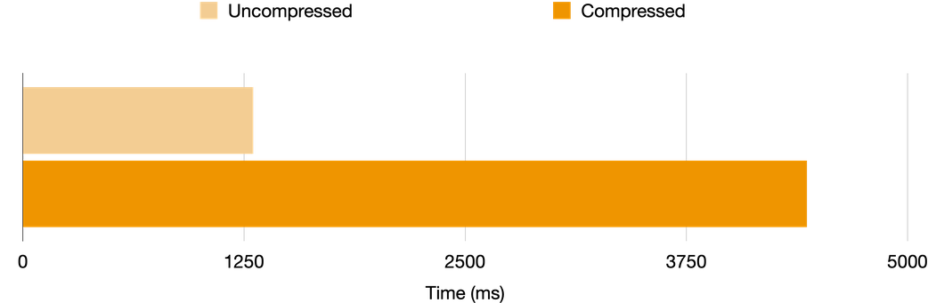
The results of this query aligns with the expected behaviour, with compressed data taking over 3 times longer. Next we test for some queries where we would expect compressed data to perform better, including:

1. Selecting older data for a particular symbol
2. Calculating TWAS (Time-Weighted Average Price) by symbol
3. Calculating basic metrics (min, max bids etc) grouped by symbol and 5-minute time buckets

These queries gave the following results:

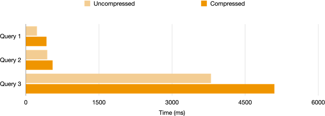
In these cases the compressed data does perform much better although still not quite as fast as the uncompressed data. Determining whether the trade-off between storage space and query performance is worthwhile relies on your specific needs, and in some cases compression can be a win-win. The capability to compress individual chunks also provides an opportunity to find a favourable balance between compressed and uncompressed data.

Conclusion

In conclusion, TimescaleDB proves to be a valuable tool for working with time series data, offering several notable advantages over PostgreSQL.

The implementation of time based partitions can significantly enhance query performance and in certain cases query speed can improve by up to 15 times, enabling more efficient data retrieval and analysis.

Hyperfunctions and continuous aggregates streamline data analysis, making it easier and more efficient. Continuous aggregates, in particular, provide a powerful mechanism for precomputing and updating aggregations in real-time, facilitating faster querying of aggregated data.

In our testing, the insert performance in TimescaleDB and PostgreSQL was largely comparable. However, we would expect Timescale to scale better and this could be a topic of further investigation.

Maybe the most impressive feature of TimescaleDB is the compression capabilities. We achieved a compression rate of over 80%, while maintaining query performance comparable to uncompressed data. This allows for very efficient utilisation of storage space without sacrificing query efficiency.