Fast, Flexible, Low Memory end-of-day writes with TorQ 2.3
Data Intellect
If you are given the option, is it to your advantage to switch on your initial choice?
The Monty Hall problem:
Suppose you’re on a game show, and you’re given the choice of three doors:
Behind one door is a car; behind the others, goats. You pick a door, say No 1, and the host, who knows what’s behind the doors, opens another door, say No. 3, which has a goat. He then says to you, “Do you want to pick door No. 2?
Is it to your advantage to switch your choice?
The end-of-day write down problem:
Suppose you have a large data capture system, say TorQ , and you need to write data down to disk on a daily basis. You have already decided you will use a WDB (write database) process, but now you have a choice on the write down scheme you will use.
You pick the default method:
- default – Data is written temporarily to disk with the same partition scheme as the HDB (historical database). At the end-of-day, data is sorted before being moved to the HDB.
But are given the choice to switch to a new optional method:
- partbyattr – Data is written to a custom partition scheme which is analagous to the default sort process. At the end-of-day, data is appended to the HDB in chunks without the need for sorting.
Is it to your advantage to switch your choice?
Solutions:
The Monty Hall problem:
The answer to the Monty Hall problem is straight forward. You should always switch!
You have a 2/3 chance of winning when you switch, versus a 1/3 chance if you don’t. I will leave it to you to read up on the proofs, solutions and controversy for this problem.
The end-of-day write down problem:
The answer to the WDB end-of-day problem requires a bit more of a discussion. The following blog discusses techniques which are similar to those outlined here , but focuses on the TorQ specific implementation and expands the discussion to include memory usage and the effect of data cardinality.
Currently within TorQ, a WDB process can be used to reduce peak memory usage and speed up the end-of-day write down. Throughout the day, data is written at regular intervals to a temporary directory and, at the end-of-day, any remaining data is flushed to disk, sorted and moved to the HDB. By default, the WDB writes to a directory structure which is similar to the HDB and defined by the partitiontype variable. Before being moved to the HDB, the data is sorted and assigned attributes according to the parameters defined in the sort.csv configuration file.
Below is a sample quote schema and corresponding sort.csv table for FX data:
date       time                 sym    side price    size     lp    quoteid
--------------------------------------------------------------------------------------------------------
2015.12.11 0D00:00:11.110868118 NZDUSD S    0.6599   5000000  FXALL 938fe46d-7a3f-6683-8f59-d3821f28aaa2
2015.12.11 0D00:01:34.767705816 EURJPY S    130.6    2000000  CURNX 491c86a1-d5d7-b8fb-54b8-951987cd1cdc
2015.12.11 0D00:02:06.964839734 USDZAR B    14.3699  10000000 HSPT  d056ea15-7339-2419-c87d-219c470eb7a7
2015.12.11 0D00:04:03.104944378 ZARJPY B    8.6      9000000  CURNX bc022112-ac46-255e-801e-6777699b5a1e
2015.12.11 0D00:04:59.182989634 CHFJPY S    120.2199 5000000  CURNX 304f4556-af09-6c43-70f6-f697a8a5eed9
...
tabname,     att,     column,     sort
default,     p,	      sym,        1
default,     ,        time,       1
quote,       p,       sym,        1
quote,       ,        time,       1
Using the default write down method, the data would be temporarily written to the WDB with the following partition structure:
/<savedir>/<partitiontype>/<tablename>/
And a typical directory tree would be similar to:
├── hdb
│   └── database
│       └── sym
└── wdb
    └── 2015.12.11
	└── quote
	    ├── lp
	    ├── price
	    ├── quoteid
	    ├── side
	    ├── size
	    ├── sym
	    └── time
...
Although the WDB process is a desirable approach compared to a standard tick set-up, the sort process can still be memory and computationally intensive.
The new partbyattr method may, for certain datasets, significantly improve the write down times and reduce memory usage further. The new method temporarily writes to a partition scheme which reflects the outcome of the end-of-day sort process and is derived from the sort.csv configuration file. Within sort.csv any columns that are defined with the `p (parted) attribute are used to generate the custom partition structure (which is analogous to the default sort process). At the end-of-day, the data is appended in manageable chunks to the HDB, without the need for sorting, and the parted attributes are applied to the appropriate columns.
Using partbyattr the data would be written to the WDB with the following partition structure:
/<savedir>/<partitiontype>/<tablename>/<parted column(s)>/
And a typical directory tree would be similar to:
├── hdb
│   └── database
│       └── sym
└── wdb
    └── 2015.12.11
        └── quote
            ├── AUDCAD
            │   ├── lp
            │   ├── price
            │   ├── quoteid
            │   ├── side
            │   ├── size
            │   ├── sym
            │   └── time
            ├── AUDCHF
            │   ├── lp
            │   ├── price
            │   ├── quoteid
            │   ├── side
            │   ├── size
            │   ├── sym
            │   └── time
            ├── AUDJPY
            │   ├── lp
            │   ├── price
            │   ├── quoteid
            │   ├── side
...
It is also possible to part on multiple columns and is easy to implement, simply by modifying the sort.csv file.
Because the partition scheme is taken from the sort.csv file, the data is already stored in the desired sorted configuration. All that is required at the end-of-day is to merge the data in chunks and apply the parted attribute. The number of rows merged at once can be set by the mergenumrows and mergenumtab variables, which can limit peak memory usage further.
Both methods will produce the same sorted tables and same partition directory in the HDB, similar to:
├── hdb
│   └── database
│       ├── 2015.12.11
│       │   └── quote
│       │       ├── lp
│       │       ├── price
│       │       ├── quoteid
│       │       ├── side
│       │       ├── size
│       │       ├── sym
│       │       └── time
│       └── sym
└── wdb
...
The new partbyattr method is recommended for large data sets with a low cardinality (small number of distinct elements). A good example where it would be beneficial is partitioning by sym on FX quote data (where there is a small number of currencies that are quoted heavily). For data sets with a larger number of distinct elements it may still be beneficial to use the partbyattr write down method, but with appropriate considerations.
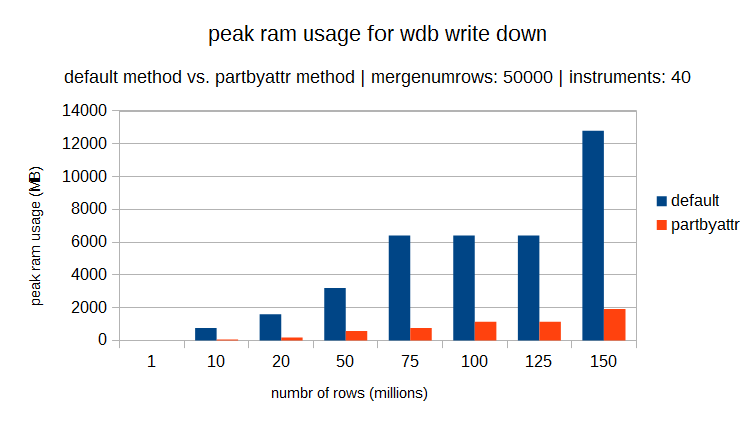
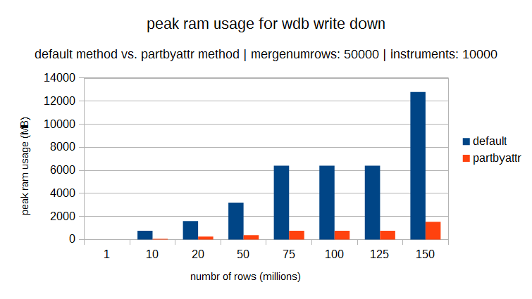
One thing is certain, the partbyattr method will greatly reduce the spike in memory at the end-of-day. The main reason for this is that the merging process is less memory intensive than sorting. The peak memory usage in the merging process is determined by size of the individual chucks being merge in one go, and this is limited using the mergenumrows and mergenumtab vaiables. The peak memory usage using the sort process is related to the total size of the table being sorted and the size of the largest column (for example a guid or character array column). The following graphs show the peak memory usage for two datasets with varying number of distinct elements (40 & 10000). For both it can be seen that the partbyattr method uses significantly less RAM than the default method.
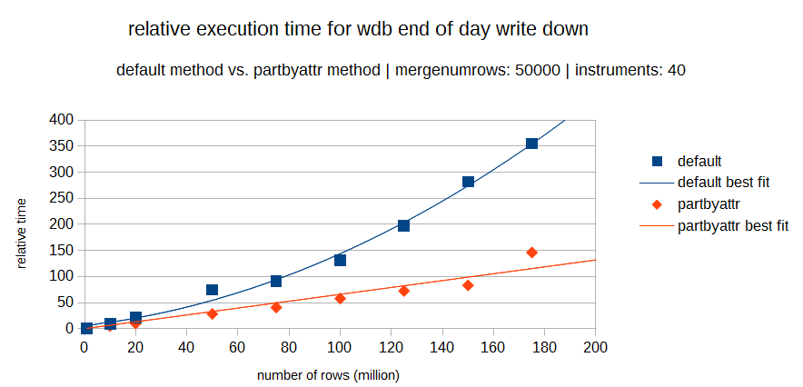
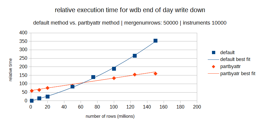
But the relative execution times between the two methods will depend heavily on the particular datasets involved. The following two graphs show how the relative times of both methods may vary. The first graph is for a dataset with a low number of distinct elements (40) and the second is a set with a higher amount of distinct elements (10000).
It can be seen in both graphs that the partbyattr method becomes increasingly faster than the default method, as the number of rows in the dataset increases. But as highlighted in the second graph, for datasets with a larger number of distinct elements, there is an important cross over between the two methods. So, for a small dataset with a large number of distinct elements, the default method will probably be preferable. This is where the cardinality ratio comes in.
But its not that simple….
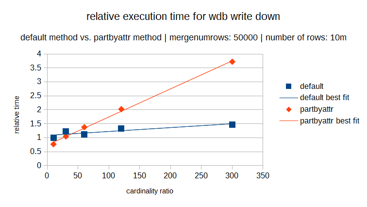
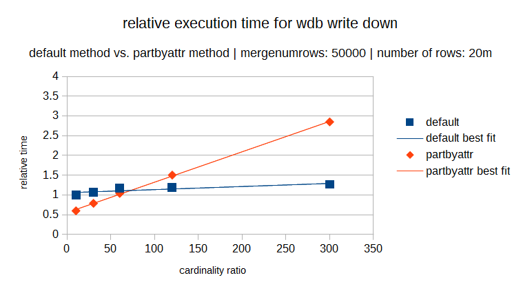
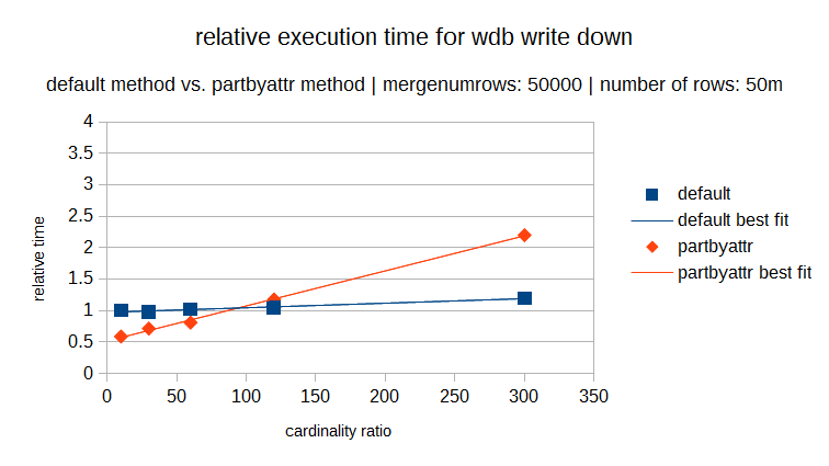
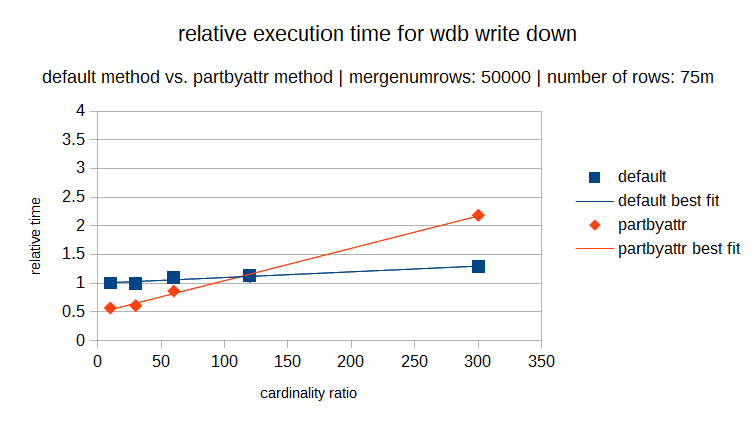
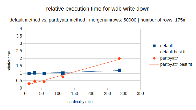
The following graphs show the execution times of both methods over the same cardinality range (where the cardinality ratio is defined as the number of rows in the dataset divided by the number of distinct elements). Each graph has a different number of rows in the dataset (and in proportion a different number of distinct elements). In each individual graph you can see the relative execution time for varying cardinality ratios and it is obvious that for lower cardinality the partbyattr method is definitely preferable.
But you can also see that as the number rows in the dataset increases, the ratio where the cross over point occurs also increases. So the cardinality rule is now also variable.
The important consideration in determining which method should be used, is on the relative performance of a systems CPU and disk I/O speed. The default write down method uses a sorting algorithm where the execution time depends more on the CPU. The partbyattr method writes and reads to disk more frequently and so the execution time is more dependent on disk I/O speed.
For our example datasets we used:
KDB: version 3.3 (2015.07.29)
CPU: Intel(R) Xeon(R) CPU E5640 @ 2.67GHz 12Mb Cache
RAM: 16 GB
DISK: RAID5 array of 7200rpm SATA disks
But the results will vary depending on different hardware configurations.
The good news is, implementing the feature is easy. All that’s required, is to specify partbyattr for the writedownoption variable in the WDB configuration, and TorQ takes care of the rest. The more difficult part is deciding whether it is desirable considering your system specifications.
So….
Now that you are presented with two write down options, which one should you use?
If you are given the option, should you switch?
Potential time savings and memory reductions are there to be had!
Maybe we could help assess your options and help you decide, if so let us know.
Share this:

