Data Intellect
One of the most requested features to our kdb+ Grafana adaptor was the ability to create panels from the results of server side functions. This most recent update to the adaptor continues to build on the SimpleJSON datasource created by Grafana by working around the limitation of the single drop down menu for queries, whilst also allowing parameters to be supplied. The adaptor is also integrated into TorQ as a whole, meaning this update will be available to any TorQ process.
Function calls can be typed directly into the query box; by adding the prefix “f” followed by the server’s chosen delimiter character (“.” by default) to the function call, the function will be executed, and if the result is a table, it can be manipulated in the same way as in-memory tables for both the table and time-series response options. Functions which do not return a table will return an error if an attempt to use them is made.
Usage
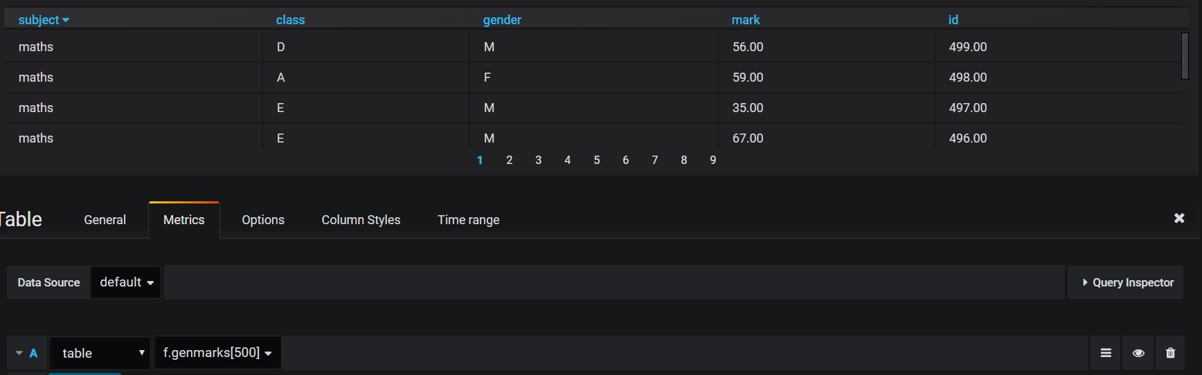
Function requests for ordinary tables take the format of “f.functionname[params]”, where parameters are supplied in exactly the same way as they would be on the server. For example, take the “f” function from the school.q script (renamed to “genmarks” here for clarity) which returns a table of randomised exam results data with x number of rows:
[code]genmarks:{([]subject:(4*x)#`maths`english`french`ict;class:raze 4#/:x?”ABCDE”;gender:raze 4#/:x?”MF”;mark:35+(4*x)?60;id:raze 4#/:til x)}[/code]
After we define this function on the server connected to Grafana, typing “f.f[500]” into the query box will call the function and return a table with 500 rows:
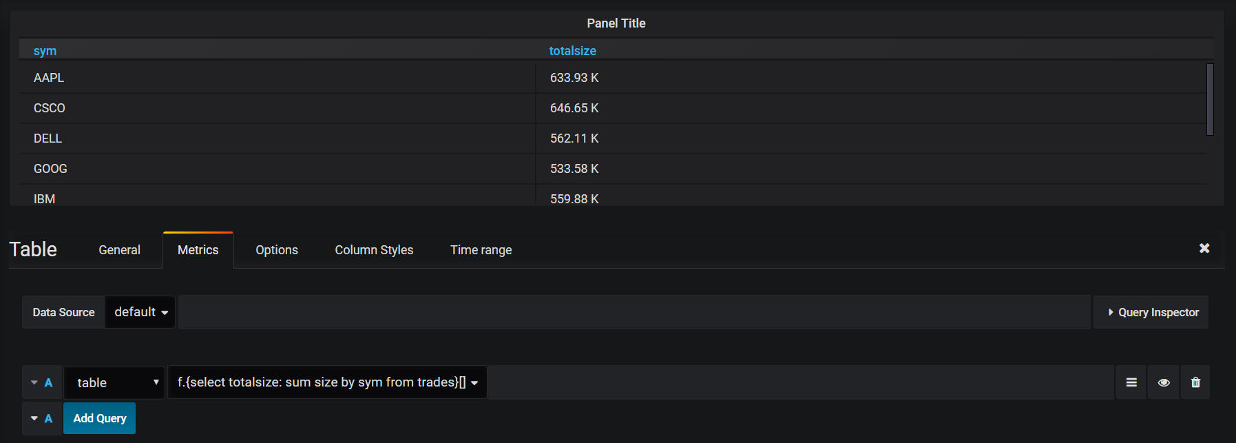
Empty square brackets are required to execute a function with no parameters. Here, the user defined function “markstats” will select certain metrics from the in-memory “marks” table, also from school.q:
[code] markstats:{select mxmark:max mark, mnmark:min mark, mdmark:med mark from marks} [/code]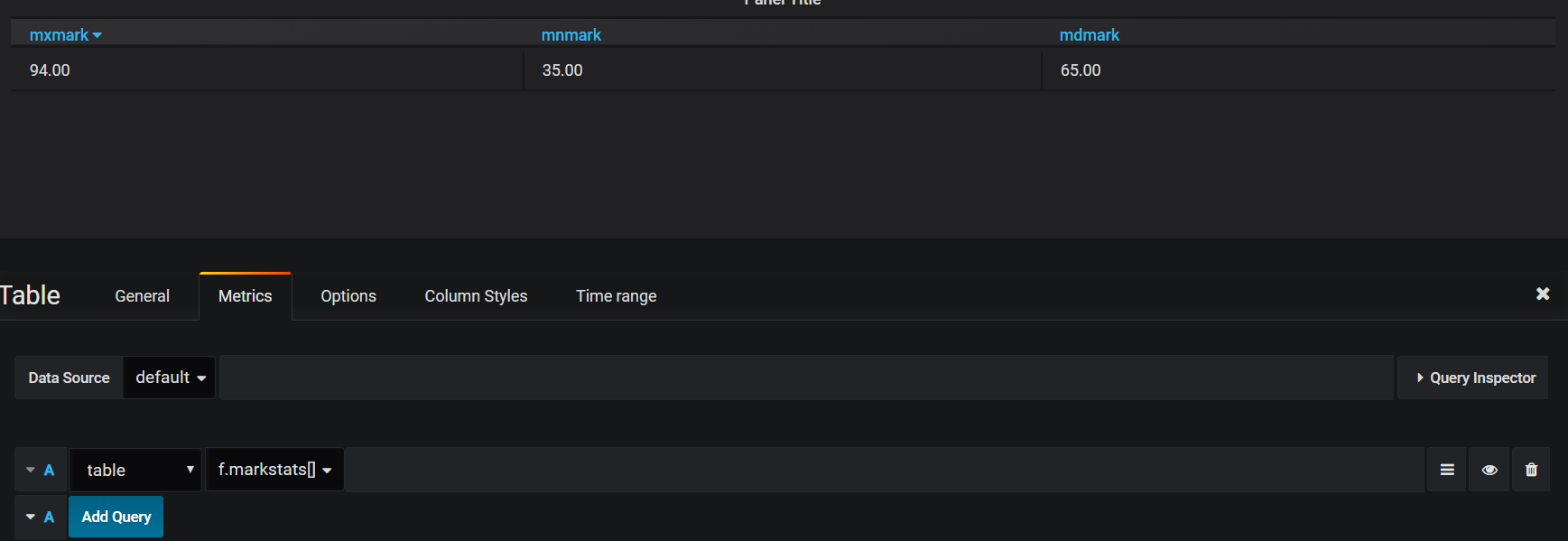
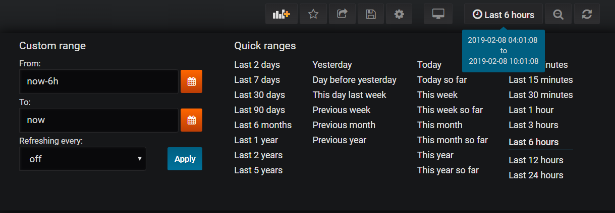
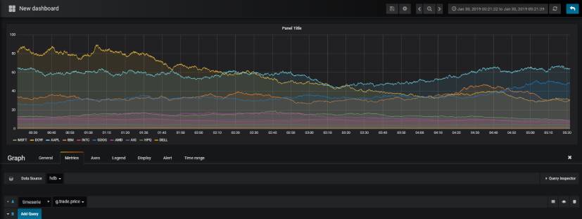
Time-series requests allow the user to narrow down queries on tables containing a time column to a certain range from within Grafana; this range can be modified by clicking the clock icon at the top right corner of the panel editor:
The format for time-series requests for functions is “f.type.functioname[params]”, where “type” refers to the current panel. As with in-memory queries, the appropriate character for each panel type must also be supplied, namely “t” for table panels, “g” for graph panels, or “o” for other panel types, such as heat-maps; this is to workaround the fact that information on the panel type, and therefore what format the data must be returned in, is not included in Grafana’s JSON request to the server.
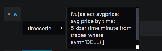
Anonymous functions can be used in place of a named function by wrapping the query to execute in curly braces followed by any parameters, again in the same way as one would on the server:
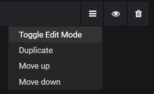
Lambdas can be combined with “t”, “g”, or “o” to create the appropriate panel in the same way as named functions. Toggling edit mode by selecting the menu button will expand the query box, which may make editing lengthy lambdas or functions with many parameters easier:
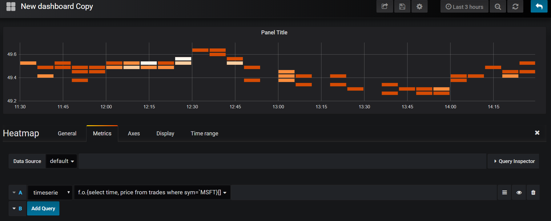
Functions which return a table containing a time-series column and a single other column can be used to create heat-maps and single stat panels. Unlike in-memory tables, no column names can be supplied after the function:
The update works by checking for the “f” prefix before the query string is parsed. If so, everything after the first instance of the user defined delimiter is executed; if a time-series request is made, the panel type character is split and collected in a similar way, so the result of the function can be sent to the correct handler. This way, parameters containing the delimiter will not be separated from the full function call, e.g floating point numbers. Otherwise, the arguments for querying an in-memory table are parsed as normal, splitting the string by each occurrence of the delimiter.
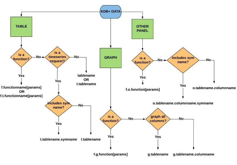
For clarity, the flowchart of valid queries for each panel type from the previous blog has now been updated to include the syntax for functions:
Namespaces
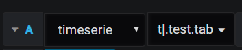
Important to note is that whilst the drop down menu does not contain tables or functions from other namespaces in the connected session, it is still possible to call them if the namespace is included before the name of the function or the table in full, and after the required prefixes e.g. for a function “func” defined in namespace “.d”, the query will look like “f..d.func[]”. However, for querying in-memory tables from other namespaces, it will be necessary to change the delimiter to something other than “.” for the query to be parsed correctly. This can be done by reassigning the “.grafana.del” variable on the connected server to the character of your choice, preferably a pipe “|”. The drop down menu will be repopulated with the same options as before, using the new delimiter; queries to the namespace will also need to use this character. As an example:
[code]q)\l grafana.q
q)\d .test
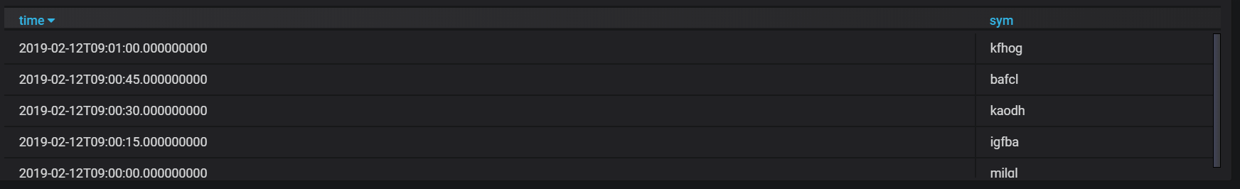
q.test)tab:([]time:09:00:00+15*til[5]; sym:5?`5)
q.test).grafana.del:”|” [/code]
HDB Support
An important addition since the initial adaptor update is the ability to read data directly from a HDB running on a TorQ process into Grafana. This can be done by simply setting the URL of your SimpleJSON datasource to the IP address of your server followed by the port your HDB is running on. Before querying your HDB, ensure your time-series range is setup correctly and that you select only the required columns; selecting too wide a range may result in crashing your HDB.
Fixes
Rows from keyed tables are now collected correctly, allowing both graph and table panels to be created:
[code] tab:([somekey:1 2 3 4 5]time: 09:00:00 + 15*til[5];sym:`A`B`C`D`E; nums: 1.2 1.3 1.4 1.5 1.6)[/code]
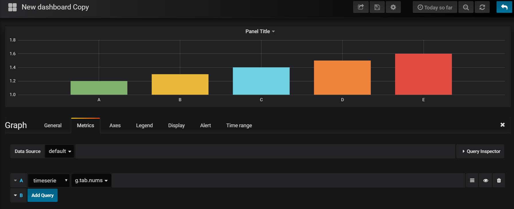
One small change has been made for usability: previously, if you selected “t.trades” or “t.trades.MSFT” for your query in a table panel, this would only work if you had also selected “timeserie” from the response dropdown; now, if you select table, this will create a table as expected, the key difference being that the Grafana time range option will not be applied.
Going Forward
Although it was possible to implement this feature within the constraints imposed by the SimpleJSON datasource, it has also exposed the adaptor’s limitations: graphs and heat-maps for non-time-series data are unable to be created from either functions or in-memory tables, and the query syntax required to return data in the correct format becomes cumbersome when working with other namespaces. AquaQ Analytics are now researching a replacement for this adaptor, which would allow for a more generalised approach to visualisation of kdb+ data, greater flexibility for queries, and provide a more user-friendly interface for supplying parameters to functions which would not require knowledge of q syntax.
Share this: