Ciaran Corvan
ClickHouse is a fast open-source column-oriented database management system for online analytical processing.
It is:
- SQL-based
- Column-oriented
- Designed for ingestion of millions of rows per second
- Designed for fast query execution
- Designed to be used with analytical workloads
Use cases typically involve capturing data related to Observability, Real-time Analytics, Data Warehousing and Machine Learning/Generative AI.
In this blog we explain some of the features of ClickHouse. Including how it stores data, what makes it fast, best practices and some of its features.
How ClickHouse Stores Data
Each table has an Engine. An Engine determines how and where the data is stored for example:
It could be a table stored locally in native ClickHouse storage:
CREATE TABLE trades(
    time Datetime64(9),
    sym LowCardinality(String)
    price Decimal64(2)
)
ENGINE = MergeTree
PRIMARY KEY (sym)
CREATE TABLE uk_property
ENGINE = S3('https://learn-clickhouse.s3.us-east-2.amazonaws.com/uk_property_prices/uk_prices.csv.zst')
PRIMARY KEY town
In the case of the S3 engine the data will not be stored anywhere other than the s3 bucket itself, same goes for any of the non-native table engines. Therefore if performance is required it is best to use the native ClickHouse storage.
MergeTrees
Consider our trade table from before:
CREATE TABLE trades(
time Datetime64(9),
sym LowCardinality(String)
price Decimal64(2)
)
ENGINE = MergeTree
PRIMARY KEY (sym)
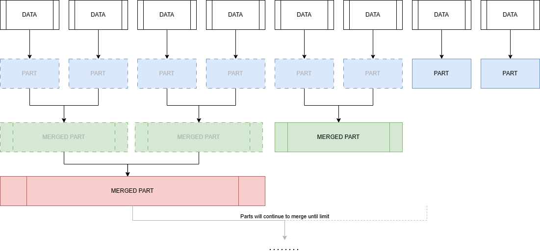
Each insert performed on the table creates a part. A part is an immutable folder containing files for each column + metadata. Over time these parts merge together and the original parts are deleted. These parts continue to merge until a set limit which is defaulted to 150GB.
This means you will want to keep inserts as large as is reasonable for your dataset. In the cases where client-side batching isn’t an option, you can use Asynchronous Inserts. These write data to an in-memory buffer and then flush to storage when configurable conditions like size, time or number of inserts are met.
The base table engine is the regular MergeTree but there are a number of other merge tree engines. These add extra functionality for specific use cases and for the most part work in the same way. The ClickHouse documentation contains a list of them here.
For Production environments not using ClickHouse cloud the Replicated* version of the mergeTree engines should be used for availability in a user environment. One thing to be aware of is if you are using ClickHouse cloud this replication is taken care for you automatically and therefore there is no need to use the replicated versions of the mergeTree engines.
Primary Keys
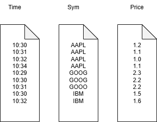
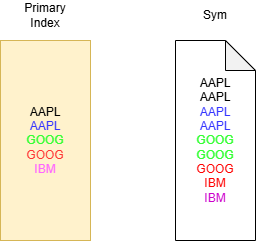
Similar to kdb+ each part contains a file for each column. Unlike kdb+ this file like the part folder it belongs to is immutable and is sorted by the primary key defined on table creation. Note, it is possible to have more that one column make up the primary key. For our trades tables it would look something like the diagram on the right:
A word on updates
As mentioned, in ClickHouse data is immutable. The system has been designed around inserts and efficiently storing data. However, there are still a number of ways to delete and update data:
- Mutations via the ALTER TABLE statement, these will completely rewrite the entire part and cannot be rolled back. ClickHouse recommends these are avoided if possible.
- Lightweight Deletes: ClickHouse creates and maintains a hidden column which marks the data to be deleted, on the next merge the rows will be dropped.
- Deduplicating merge trees: These include ReplacingMergeTree for Upserts and infrequent updates, CollapsingMergeTree for frequent updates and VersionedCollapsingMergeTree for frequent parallel updates.
Speed in ClickHouse
One of the design features of ClickHouse making queries fast is its ability to avoid full table scans when possible. This is done by splitting parts into Granules.
In ClickHouse a Granule is a collection of rows used to scale query processing. The default number is 8192 and usually doesn’t need to be changed.
At query time each part in a table can be viewed as a collection of granules to be processed. This creates a primary index with one key per granule. If queries use the primary key as a filter, this will allow for the skipping of granules. In the example above if we were to set the number of rows in a granule to 2 and run
SELECT avg(price) from trades where sym=`GOOG
Only the Green and Red rows are processed. These will then be sent to separate threads for processing.
Choosing Primary Keys
It is hopefully clear that the primary key is probably one of the most important considerations when designing a table schema. For kdb+ folks this is analogous to the `p# attribute on a HDB.
If you would like multiple primary indexes then ClickHouse has a number of solutions:
- Projections: ClickHouse creates a hidden table storing data sorted differently, possibly with some aggregations or data transformations. At query time the request is sent to the hidden table if it allows for a more efficient execution. Originally this meant storing data twice if you create a projection with different primary key, however in a recent update projections can now be set to behave like a secondary index.
- Materialized Views: Data is stored in a separate table based on a SELECT statement.
- Skipping index: Metadata about the blocks of data are stored, allowing for ClickHouse to infer if those blocks need to be read or not.
ClickHouse Features
ClickHouse supports most ANSI SQL queries including GROUP BY, ORDER BY, WITH, JOINS etc, there are a number of other features worth mentioning. Note this is by no means an exhaustive list.
Optimizing Joins
At the time of writing Clickhouse has six different join algorithms as an additional option for JOIN statements. These can be set as part of the SELECT JOIN statement, they are:
- direct
- parallel_hash
- hash
- full_sorting_merge: Normal sort-merge join
- grace_hash
- partial_merge
The choice depends on performance, memory and Join type support. Selecting the correct one is a non-trival matter. A great blog post from ClickHouse goes into detail on how to select the correct algorithm. If you’re not too bothered then you can set the join_algorithm to auto which will allow ClickHouse to try parallel hash joins , switching on the fly to partial merge join if the algorithm’s memory limit is reached.
Materialized Views
In ClickHouse there are two main types of materialized views:
- Refreshable: where the target table SELECT statement is executed periodically.
- Incremental: where the SELECT is run on the inserted rows before adding to the target table.
In the context of Incremental materialized views you might ask “what about aggregations?” In this case the AggregatingMergeTree Engine is a special mergeTree with aggregation state datatypes like AggregateFunction(avg UInt32). These store the intermediate “states” of an aggregation and can be merged at query time in order to compute the final aggregation.
Compression
ClickHouse has a number of nice features to reduce the size of the database:
- DataTypes like LowCardinality(String) which store strings as integers working much the same way as kdb+ enumeration.
- Delta-based Codecs.
- Time-To-Live (TTL) an out of the box way to delete data once it reaches a certain age.
- Column-wise compression.
ASOF Joins
ClickHouse supports ASOF joins:
select * from t
┌────────────────────time─┬─sym─┬─qty─┐
1. │ 2026-03-04 14:45:43.000 │ a │ 100 │
2. │ 2026-03-04 14:45:39.000 │ c │ 150 │
3. │ 2026-03-04 14:45:27.000 │ b │ 200 │
└─────────────────────────┴─────┴─────┘
select * from q
┌────────────────────time─┬─sym─┬─price─┐
1. │ 2026-03-04 14:45:35.000 │ a │ 98  │
2. │ 2026-03-04 14:45:17.000 │ b │ 99  │
3. │ 2026-03-04 14:45:31.000 │ b │ 101 │
4. │ 2026-03-04 14:45:08.000 │ a │ 100 │
└─────────────────────────┴─────┴───────┘

SELECT
time,
sym,
qty,
price
FROM t
ASOF LEFT JOIN q ON (t.sym = q.sym) AND (t.time >= q.time)

┌────────────────────time─┬─sym─┬─qty─┬─price─┐
1. │ 2026-03-04 14:45:27.000 │ b │ 200 │ 99   │
2. │ 2026-03-04 14:45:39.000 │ c │ 150 │ 0    │
3. │ 2026-03-04 14:45:43.000 │ a │ 100 │ 98   │
└────────────────────────────┴───┴─────┴──────┘
Notice that the price here is 0 but it probably should be NULL. In ClickHouse null values are stored as their default values. If you want the data to actually be null then the Nullable datatype will need to be used. In this case a hidden column is created which will be read if required, say for example if you wanted the average price for the above table without nullable you get ~65.67. If it was the nullable datatype you’d get 98.5. Nullable types bloat your dataset so it is best to avoid them if possible.
Rounding up
While this is certainly not a comprehensive overview of ClickHouse, hopefully you have been able to take away an idea of how it works and some of the features in it. There is a lot of interesting ideas in some of the design choices for data storage. We will be continuing to explore ClickHouse, in particular how it fits into the timeseries and kdb+ finance world.
Thanks for reading!
Share this: