An Introduction to QuestDB

Introduction

Working with financial time-series data, you will encounter a recurring set of problems that general-purpose SQL databases handle poorly. Trades and quotes arrive at different frequencies and need to be aligned. Tick data accumulates quickly and needs to be stored cheaply without sacrificing queryability or durability. Dashboards need the most recent value per instrument without scanning an entire table. QuestDB is a database focussed on solving these problems.

Covered in this blog:

• Ingestion architecture: ILP over HTTP and TCP, WAL-based durability
• Three-tier storage: hot WAL, warm columnar binary, cold Parquet
• Finance-inspired timeseries SQL extensions: ASOF JOIN, HORIZON JOIN, WINDOW JOIN, SAMPLE BY
• Exchange calendar support
• Materialised views
• Language and protocol integrations
• What we like about QuestDB
• Room for improvement

Background

QuestDB was created specifically for financial time-series data. Development began in 2014, with the open-source release under Apache 2.0 following in 2019. Y Combinator backed the project in 2020. Since then they’ve accrued a number of users in industry. The project is actively maintained, with releases approximately every three weeks.

Key Features

Ingestion

The recommended ingestion path for high throughputs is the InfluxDB Line Protocol, aka ILP. SQL INSERT and message brokers such as Kafka are also supported along with importing from CSV and Parquet. ILP supports both HTTP and TCP. Both have specific use cases with HTTP being the recommended approach and TCP being typically used in legacy QuestDB versions or situations with high network latency. The reasoning for HTTP being preferred is error reporting, retry logic and transaction control. The main bottleneck of HTTP is that each flush will block until the server acknowledges the request, on deployments where the database and writer are on the same LAN the block can be sub-millisecond so it can be trivial in a lot of cases, although not all use cases.

QuestDB does not keep data resident in memory. Data arriving via ILP is first written to a Write-Ahead Log (WAL), which allows multiple concurrent writers without blocking one another. The WAL is then applied to the main columnar storage in the background by a component called the TableWriter. Once applied, data becomes queryable. How quickly that happens depends on the WAL apply cycle speed, out-of-order (O3) patterns, and configuration parameters.

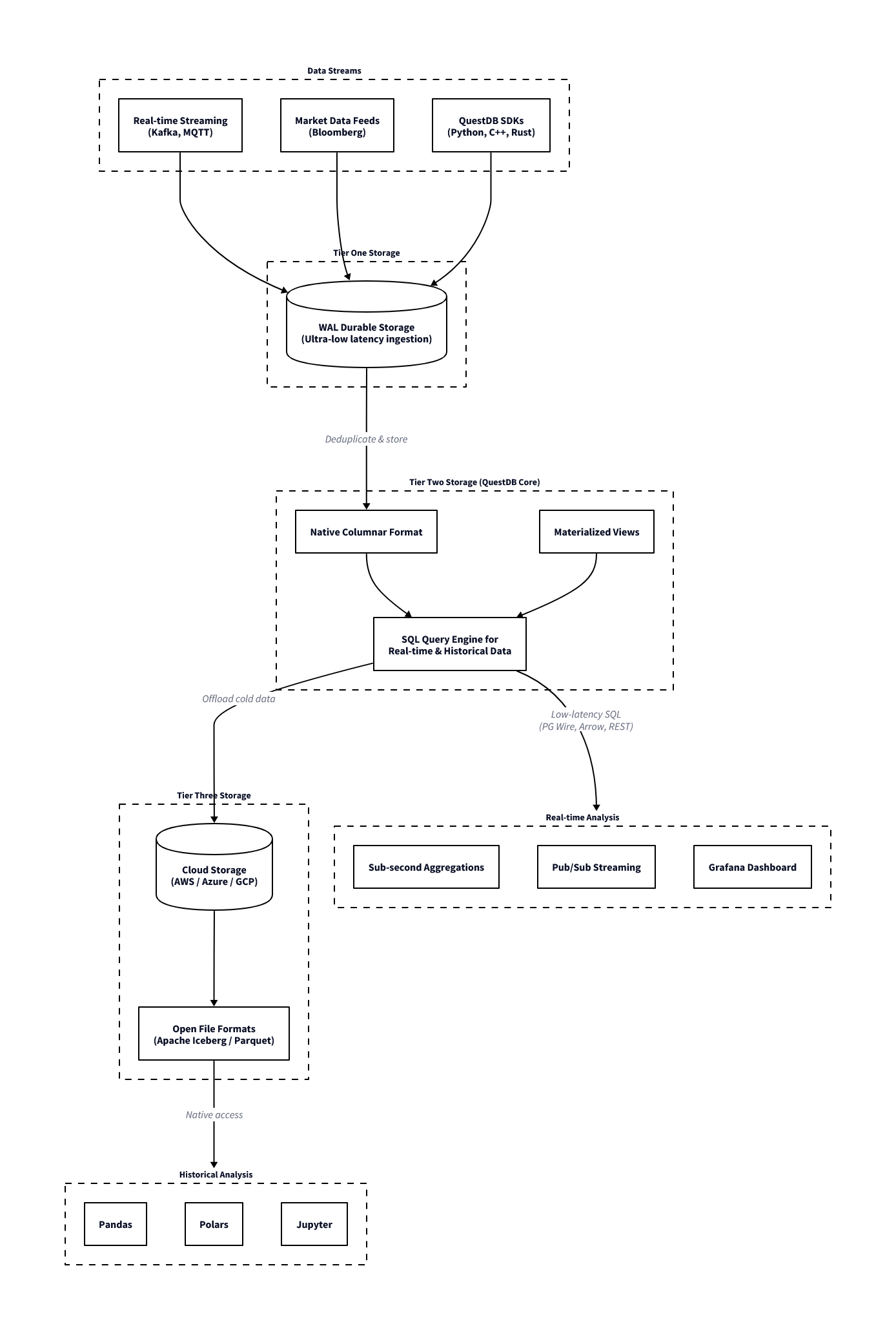
Storage Tiers

QuestDB organises data across three tiers, each with different characteristics for write latency, query performance, and storage cost. This explains why the database is fast on recent data and how it handles long historical archives.

The first tier is the Write-Ahead-Log (hot storage). Each connection maintains its own WAL file, so concurrent ingestion does not require table-wide locking. A Sequencer component coordinates consistency across readers during writes.

Once the WAL has been applied, the data moves to the second tier: QuestDB’s native columnar binary format (warm storage). This is the primary query layer: column files are memory-mapped, vectorised operations run directly over them, and out-of-order writes and deduplication are handled at this stage. Recent partitions reside here.

The third tier is Parquet (cold storage). Older partitions can be converted to Parquet format, which reduces storage cost through better compression and makes the data accessible to external tooling such as Spark, DuckDB, or any other Parquet-compatible reader, without requiring a separate export step. In QuestDB Enterprise, this conversion and movement to object storage (S3, GCS, Azure Blob) happens automatically as partitions age.

For queries, the planner spans the columnar binary and Parquet tiers. The WAL is a write path and data only becomes queryable once applied to columnar storage. A single SQL query over a multi-year dataset will read recent data from binary column files and older data from Parquet (on local disk or object storage) without any syntax difference or manual union required. From the perspective of the query, the storage location of a partition is not visible.

QuestDB ingestion and storage architecture

ASOF Joins

Two time-series you want to combine often don’t tick at the same frequency. Trades arrive at irregular intervals while quotes update independently, and order events don’t align with market snapshots. To attach the correct quote to each trade (the quote prevailing at the exact moment of execution), you need the most recent quote with a timestamp at or before the trade timestamp.

SELECT t.time, t.sym, t.price, t.size,
       q.bid, q.ask
FROM trades t
ASOF JOIN quotes q ON (sym)

time	sym	price	size	bid	ask
2024-01-15T09:30:00.100000Z	AAPL	185.5	100	185.48	185.58
2024-01-15T09:30:00.150000Z	AAPL	185.55	200	185.5	185.6
2024-01-15T09:30:00.200000Z	MSFT	375.2	150	375.15	375.25
2024-01-15T09:30:01.000000Z	AAPL	185.6	300	185.55	185.65
2024-01-15T09:30:01.100000Z	GOOGL	141.8	250	141.75	141.85
2024-01-15T09:30:01.200000Z	MSFT	375.25	100	375.18	375.28
2024-01-15T09:30:02.000000Z	AAPL	185.45	500	185.58	185.68
2024-01-15T09:30:02.100000Z	GOOGL	141.85	175	141.78	141.88
2024-01-15T09:31:00.000000Z	AAPL	185.7	400	185.42	185.52
2024-01-15T09:31:00.100000Z	MSFT	375.3	200	375.22	375.32

In most SQL databases, this is verbose and slow, requiring window functions, lateral joins, or application-layer workarounds. In QuestDB, this is supported natively within the query engine.

Use cases:

• Attaching prevailing bid/ask to each execution for cost analysis
• Aligning order events to the most recent market snapshot
• Joining two independently-sourced price series that tick at different frequencies
• Computing effective spread at time of execution

HORIZON JOIN

HORIZON JOIN extends the ASOF join concept to allow for analysis at fixed time points around an event. This is especially used in “markout” analysis in trading. Markout analysis measures how a price or metric evolves after (or before) an event, such as a trade. This is commonly used to analyse the PnL evolution around a trade, and when viewed on aggregate across all trades allows decisions to be made on how to handle the risk associated with trading broken down by different classifications, such as instrument, counterparty, time of day, etc.

Two forms are available depending on whether the intervals are regular or not. The RANGE form generates offsets at uniform steps:

SELECT
    t.sym,
    h.offset / 1000000 AS horizon_sec,
    avg((q.bid + q.ask) / 2) AS avg_mid
FROM trades t
HORIZON JOIN quotes q ON (sym)
RANGE FROM 0s TO 5m STEP 1m AS h
ORDER BY t.sym, horizon_sec;

sym	horizon_sec	avg_mid
AAPL	0	185.556
AAPL	60	185.7
AAPL	120	185.7
AAPL	180	185.7
AAPL	240	185.7
AAPL	300	185.7
GOOGL	0	141.815
GOOGL	60	141.87
GOOGL	120	141.87
GOOGL	180	141.87
GOOGL	240	141.87
GOOGL	300	141.87
MSFT	0	375.2333
MSFT	60	375.33
MSFT	120	375.33
MSFT	180	375.33
MSFT	240	375.33
MSFT	300	375.33

This produces a result for each offset (0s, 1m, 2m, 3m, 4m, 5m), showing the average mid-price from the quotes table at each point relative to the trade timestamp. Note that h.offset is returned in microseconds; in these examples we convert it to seconds. The LIST form accepts explicit offsets, which is useful when the relevant intervals are non-uniform:

SELECT
    t.sym,
    h.offset / 1000000 AS horizon_sec,
    avg((q.bid + q.ask) / 2) AS avg_mid
FROM trades t
HORIZON JOIN quotes q ON (sym)
LIST (1s, 5s, 30s, 1m, 5m) AS h
ORDER BY t.sym, horizon_sec;

sym	horizon_sec	avg_mid
AAPL	1	185.606
AAPL	5	185.516
AAPL	30	185.516
AAPL	60	185.7
AAPL	300	185.7
GOOGL	1	141.85
GOOGL	5	141.87
GOOGL	30	141.87
GOOGL	60	141.87
GOOGL	300	141.87
MSFT	1	375.2767
MSFT	5	375.2900
MSFT	30	375.2900
MSFT	60	375.33
MSFT	300	375.33

The computation runs in a single query pass rather than requiring multiple self-joins or pivots in application code. Negative offsets are supported, so pre-trade baselines can be included in the same query for comparison. Note that HORIZON JOIN cannot be combined with other joins at the same query level, and window functions cannot be used within a HORIZON JOIN query. Beyond markout, the same pattern applies to event studies and price impact measurement for large orders across fixed reversion intervals.

WINDOW JOIN

WINDOW JOIN aggregates all rows from a second table that fall within a defined time window around each row of the first. The window is specified relative to each left-side timestamp using a RANGE BETWEEN clause:

SELECT
    t.sym,
    t.time,
    t.price,
    avg(q.bid) AS avg_bid,
    avg(q.ask) AS avg_ask,
    avg(q.ask - q.bid) AS avg_spread,
    count() AS quote_count
FROM trades t
WINDOW JOIN quotes q ON (sym)
    RANGE BETWEEN 1 second PRECEDING AND 1 second FOLLOWING
    EXCLUDE PREVAILING;

sym	time	price	avg_bid	avg_ask	avg_spread	quote_count
AAPL	2024-01-15T09:30:00.100000Z	185.5	185.51	185.61	0.1000	3
AAPL	2024-01-15T09:30:00.150000Z	185.55	185.5275	185.6275	0.1000	4
MSFT	2024-01-15T09:30:00.200000Z	375.2	375.1433	375.2433	0.1000	3
AAPL	2024-01-15T09:30:01.000000Z	185.6	185.5275	185.6275	0.1000	4
GOOGL	2024-01-15T09:30:01.100000Z	141.8	141.765	141.865	0.1000	2
MSFT	2024-01-15T09:30:01.200000Z	375.25	375.2000	375.3000	0.1000	2
AAPL	2024-01-15T09:30:02.000000Z	185.45	185.5000	185.6000	0.1000	2
GOOGL	2024-01-15T09:30:02.100000Z	141.85	141.8000	141.9000	0.1000	2
AAPL	2024-01-15T09:31:00.000000Z	185.7	185.65	185.75	0.1000	1
MSFT	2024-01-15T09:31:00.100000Z	375.3	375.28	375.38	0.1000	1

This returns, for each trade, the average bid and ask across all quotes within a ±1 second window centred on the trade time. The window can be asymmetric — backward-only for lookback analysis, forward-only for impact measurement, or both.

Use cases:

• Average quoted spread around each execution
• Volume-weighted mid-price in the seconds before an order
• Order book depth within a window around each fill

The INCLUDE PREVAILING / EXCLUDE PREVAILING modifier controls behaviour at the window boundary. EXCLUDE PREVAILING includes only rows strictly within the defined window. INCLUDE PREVAILING additionally pulls in the most recent right-side row with a timestamp at or before the window start, which is useful when the right-side series has gaps and you still want a last-known value rather than a null result.

Aggregate functions available over the matched right-side rows are sum, avg, count, min, max, first, and last. When the join key is a SYMBOL column, the engine applies a Fast Join optimisation using SIMD vectorisation across the matched rows.

SAMPLE BY

Standard SQL time-based aggregations use GROUP BY DATE_TRUNC('minute', time), which is functional but verbose and not always well-optimised by general-purpose query planners for time-series workloads. QuestDB provides SAMPLE BY as a dedicated clause for this purpose:

SELECT sym,
       SUM(price * size) / SUM(size) AS vwap,
       SUM(size) AS total_volume,
       count() AS trade_count
FROM trades
SAMPLE BY 1m ALIGN TO CALENDAR

sym	vwap	total_volume	trade_count
AAPL	185.5136	1100	4
MSFT	375.22	250	2
GOOGL	141.8206	425	2
AAPL	185.7	400	1
MSFT	375.3	200	1

By default, SAMPLE BY uses ALIGN TO CALENDAR, aligning buckets to wall-clock boundaries. A timezone can be specified with ALIGN TO CALENDAR TIMEZONE 'Europe/London' to align to local market hours, and an offset can shift the boundary to a non-standard start time. ALIGN TO FIRST OBSERVATION is also available when you want buckets to start from the first data point rather than a calendar boundary.

Use cases:

• OHLCV bar generation at any frequency
• VWAP and TWAP calculations over configurable intervals
• Volume profiles by time-of-day bucket

Exchange Calendars

Trading sessions do not map cleanly onto calendar days. Exchanges observe holidays, have early closes, and in some cases have multiple sessions within a single day with gaps in between. The standard approach to handling this is to maintain a separate calendar table and join against it, or to pre-filter data in application code before it reaches the database. Both approaches add complexity and are easy to get wrong, for example by forgetting that a particular exchange closes early on a given date.

QuestDB’s exchange calendar support (an enterprise feature) solves this by accounting for trading calendars in queries natively. Simply append an ISO 10383 MIC code to the date expression.

SELECT sym, count(), sum(size)
FROM trades
WHERE time IN '2025-01-[01..31]#XNYS'
SAMPLE BY 1d;

The #XNYS suffix restricts the interval to NYSE trading sessions only. Holidays such as Good Friday, Thanksgiving and Christmas and similar closures are dropped from results without needing to be listed. Early closes such as the July 3rd half-session are applied at the correct duration. Exchanges with multiple daily sessions, such as Hong Kong’s pre-market and afternoon sessions separated by a lunch break, are handled natively.

Built-in schedules for major exchanges are shipped as a Parquet file inside the QuestDB Enterprise JAR. On each startup this file is extracted and the schedules become available immediately — no separate download or update step is required. The file is overwritten on restart, so any manual edits to it are discarded. Custom schedules can be defined in the _tick_calendars_custom table; these are merged with the built-in data at query time and take precedence where both define the same session.

Materialised Views

QuestDB supports materialised views that maintain running aggregations as data arrives. This avoids re-scanning raw tick data each time a dashboard requests a VWAP or bar summary. Queries are defined once and QuestDB incrementally updates the result as new rows are ingested.

A running VWAP summary by symbol and minute:

CREATE MATERIALIZED VIEW IF NOT EXISTS vwap_summary_mv AS
SELECT
    time,
    sym,
    SUM(price * size) AS total_pv,
    SUM(size) AS total_volume,
    count() AS trade_count,
    SUM(price * size) / SUM(size) AS vwap
FROM trades
SAMPLE BY 30s;

select * from vwap_summary_mv;

time	sym	total_pv	total_volume	trade_count	vwap
2024-01-15T09:30:00.000000Z	AAPL	204065.0	1100	4	185.5136
2024-01-15T09:30:00.000000Z	MSFT	93805.0	250	2	375.22
2024-01-15T09:30:00.000000Z	GOOGL	60273.75	425	2	141.8206
2024-01-15T09:31:00.000000Z	AAPL	74280.0	400	1	185.7
2024-01-15T09:31:00.000000Z	MSFT	75060.0	200	1	375.3

As trades are ingested, the vwap_summary_mv table is updated automatically.

Language Support

QuestDB has two distinct language integration options. The PostgreSQL wire protocol handles querying: any language or tool with a PostgreSQL driver can connect to port 8812 (default) and issue SQL without modification. The ILP path handles high-throughput ingestion: QuestDB provides first-party clients for this in most languages commonly used in financial systems (Python, C++, etc.).

For querying, QuestDB implements the PostgreSQL wire protocol and so existing Python tooling connects without modification:

import psycopg2
conn = psycopg2.connect(host='localhost', port=8812, dbname='qdb')
cur = conn.cursor()
cur.execute("""
    SELECT sym, SUM(price * size) / SUM(size) AS vwap
    FROM trades
    SAMPLE BY 1m
""")
print(cur.fetchall())

For ingestion from Python, the dedicated client writes directly via ILP rather than through the SQL interface:

import questdb.ingress as qi
from datetime import datetime

with qi.Sender('localhost', 9009) as sender:
    sender.row('trades',
        symbols={'sym': 'AAPL', 'exchange': 'NASDAQ'},
        columns={'price': 185.50, 'size': 100},
        at=datetime(2024, 1, 15, 9, 30, 0, 100000))
    sender.flush()

QuestDB provides official ILP client libraries for Go, Java, Rust, C, C++, .NET, and Node.js. The C and C++ libraries are built on top of the same Rust implementation and expose C++11 and C++17 APIs respectively, useful for teams writing feed handlers or order management systems at the system level. The Go client is commonly used for infrastructure components.

Any language with a PostgreSQL driver works for querying without additional setup. This includes psycopg2 and asyncpg in Python, pgx and database/sql in Go, pgjdbc in Java, npgsql in .NET, and node-postgres in Node.js. Switching an existing application from PostgreSQL to QuestDB for time-series queries typically requires only a connection string change.

Getting Started

QuestDB ships with a built-in web console. Run it via Docker:

docker run -d --name questdb \
  -p 9000:9000 -p 8812:8812 -p 9009:9009 \
  questdb/questdb:latest

# Web console: http://localhost:9000
# PostgreSQL wire: port 8812
# ILP ingestion: port 9009

The web console at port 9000 is suitable for ad-hoc queries and exploration. Port 8812 speaks the PostgreSQL wire protocol, meaning psql, DBeaver, psycopg2, JDBC, and Grafana all connect without modification. Port 9009 accepts high-speed ILP ingestion.

A Practical Financial Example

To create tables:

CREATE TABLE trades (
    time TIMESTAMP,
    sym SYMBOL capacity 256 cache,
    price DOUBLE,
    size LONG,
    exchange SYMBOL capacity 32 cache
) TIMESTAMP(time)
PARTITION BY DAY WAL;

CREATE TABLE IF NOT EXISTS quotes (
    time TIMESTAMP,
    sym SYMBOL capacity 256 cache,
    bid DOUBLE,
    ask DOUBLE
) TIMESTAMP(time) PARTITION BY DAY WAL;

A few details: SYMBOL is QuestDB’s native dictionary-encoded string type, analogous to kdb+’s symbol type and ClickHouse’s LowCardinality(String). The TIMESTAMP(time) designation tells the database which column drives time-series ordering. PARTITION BY DAY WAL creates daily partitions with write-ahead logging enabled for concurrent ingestion.

With the tables created, we can insert some sample data that we will use for examples throughout:

INSERT INTO trades VALUES
    ('2024-01-15T09:30:00.100000Z', 'AAPL', 185.50, 100, 'NASDAQ'),
    ('2024-01-15T09:30:00.150000Z', 'AAPL', 185.55, 200, 'NASDAQ'),
    ('2024-01-15T09:30:00.200000Z', 'MSFT', 375.20, 150, 'NASDAQ'),
    ('2024-01-15T09:30:01.000000Z', 'AAPL', 185.60, 300, 'NYSE'),
    ('2024-01-15T09:30:01.100000Z', 'GOOGL', 141.80, 250, 'NASDAQ'),
    ('2024-01-15T09:30:01.200000Z', 'MSFT', 375.25, 100, 'NYSE'),
    ('2024-01-15T09:30:02.000000Z', 'AAPL', 185.45, 500, 'NASDAQ'),
    ('2024-01-15T09:30:02.100000Z', 'GOOGL', 141.85, 175, 'NYSE'),
    ('2024-01-15T09:31:00.000000Z', 'AAPL', 185.70, 400, 'NASDAQ'),
    ('2024-01-15T09:31:00.100000Z', 'MSFT', 375.30, 200, 'NYSE');

INSERT INTO quotes VALUES
    ('2024-01-15T09:29:59.000000Z', 'AAPL',  185.45, 185.55),
    ('2024-01-15T09:29:59.500000Z', 'MSFT',  375.10, 375.20),
    ('2024-01-15T09:29:59.800000Z', 'GOOGL', 141.70, 141.80),
    ('2024-01-15T09:30:00.050000Z', 'AAPL',  185.48, 185.58),
    ('2024-01-15T09:30:00.120000Z', 'AAPL',  185.50, 185.60),
    ('2024-01-15T09:30:00.180000Z', 'MSFT',  375.15, 375.25),
    ('2024-01-15T09:30:00.500000Z', 'MSFT',  375.18, 375.28),
    ('2024-01-15T09:30:00.900000Z', 'AAPL',  185.55, 185.65),
    ('2024-01-15T09:30:01.050000Z', 'GOOGL', 141.75, 141.85),
    ('2024-01-15T09:30:01.150000Z', 'AAPL',  185.58, 185.68),
    ('2024-01-15T09:30:01.500000Z', 'MSFT',  375.22, 375.32),
    ('2024-01-15T09:30:01.800000Z', 'GOOGL', 141.78, 141.88),
    ('2024-01-15T09:30:02.050000Z', 'AAPL',  185.42, 185.52),
    ('2024-01-15T09:30:02.200000Z', 'GOOGL', 141.82, 141.92),
    ('2024-01-15T09:31:00.050000Z', 'AAPL',  185.65, 185.75),
    ('2024-01-15T09:31:00.150000Z', 'MSFT',  375.28, 375.38);

VWAP by minute using SAMPLE BY:

SELECT
    sym,
    SUM(price * size) / SUM(size) AS vwap,
    SUM(size) AS total_volume,
    count() AS trade_count
FROM trades
SAMPLE BY 1m;

Daily OHLCV bars using first() and last():

SELECT
    sym,
    first(price) AS open,
    max(price) AS high,
    min(price) AS low,
    last(price) AS close,
    sum(size) AS volume
FROM trades
SAMPLE BY 1d;

QuestDB’s first() and last() functions respect the designated timestamp ordering, returning the chronologically first and last values within each bucket.

AI-Native

QuestDB’s standard SQL, PostgreSQL wire protocol, REST API, and open file formats such as Parquet make it straightforward for AI agents to work with. The documentation is structured around concrete use cases, which allow AI agents to work with it without much hand-holding.

Skills for Claude Code and OpenAI Codex are available; these provide QuestDB-specific query syntax, ingestion patterns, and common configurations.

Conclusion

There’s a lot to like:

• ASOF JOIN, HORIZON JOIN, and WINDOW JOINs are crucial for financial analytics and not convenient in standard SQL
• Consideration for common problems in financial domain such as exchange calendar handling
• The three-tier storage model: WAL ensures durability while recent data is fast to query, older data compresses well with Parquet and stays accessible without a separate export pipeline.
• Parquet as the cold storage format is portable and compressed, aligns to open data format principles
• The PostgreSQL wire protocol means no new client libraries are required for querying in a lot of cases
• Container-based deployment makes getting started easy and quick
• A lot of thought has gone into how agentic workflows will interact with it
• Pace of development is high, with frequent releases of new features and a public roadmap.
• Enterprise options

We are continuing to explore QuestDB and its ability around the timeseries workloads that we are used to dealing with.