Calculating VaR using Monte Carlo Simulation
Data Intellect
The need for Monte Carlo
Monte Carlo simulation is a stepwise approach to solving problems that due to the presence of some uncertainty, may not have a single answer. One such uncertainty in finance and investment is volatility. Volatility will create situations where investors might have an expected return on an investment but due to the volatile nature of markets, that expectation may overshoot or undershoot anticipated returns. Analysts often model volatility using standard deviation.
A Monte Carlo simulation is performed by running many thousands or even tens of thousands of calculations or simulations with inputs taken at random from a predetermined distribution having a specific std deviation. This allows analysts to make probability statements such as “we expect that in 99% of cases the return over 10 years will be at least 50%” or “there is a 5% chance that this investment will lose money in the next 3 months”
This post assumes the reader having a simple working knowledge of the following topics from python, finance, data science and simple statistics.
DataFrames, Collections and Comprehensions, User Defined Functions, Volatility Standard Deviation, Distributions, Value-At-Risk
Supporting Python Code
Supporting material containing jupyter notebooks for this post can be found in here .
Monte Carlo used to calculate pension fund return
Imagine you have $100,000 to invest in an ETF and you plan to retire in 30 year’s time. How much would you expect to have in your retirement account assuming you can achieve 9.5% growth each year.
Deterministic Approach
This is a simple compound interest calculation a simple formula and some python code is shown

A = final amount
P = initial principal balance
r = interest rate
n = number of times interest applied per time period
t = number of time periods elapsed
A simple python implementation of this equation might be
def compound(principal, rate, time, n = 1):
    return principal * (1 + rate/n) ** (time*n)

present_value = 100000
expected_return = .095
time_horizon = 30

ending_balance = compound(present_value, expected_return, time_horizon)
print("{:,.0f}".format(ending_balance))
With output 1,555,031
An iterative approach showing the cumulative effect of compounding could be coded as
ending_balance = 0
curr_balance = present_value

print("{:10s} {:15s}".format("Year", "Ending Balance"))
print("-" * 26)
for year in range(1, time_horizon + 1):
    ending_balance = curr_balance * (1 + expected_return)
    print("{:<10d} {:15,.0f}".format(year, ending_balance))
    curr_balance = ending_balance
Year       Ending Balance
--------------------------
1                  109,500
2                  119,902
  ....................
  ....................
29               1,389,983
30               1,522,031
Note this is deterministic, no matter how many times the above code is executed, it will always produce the same result.
Non-Deterministic Approach
The question however is can we reliably get 9.5% per year every year in the stock market. The answer is clearly no. Over a 30-year period, there will be good years and bad years, we need to incorporate volatility into the model.
The code below is very similar to the compounded interest example above but note the use of numpy.random.normal() – this function chooses a value at random from a normal distribution curve with specific standard deviation.
import numpy.random as npr

volatility = .185

ending_balance = 0
curr_balance = present_value

print("{:10s}  {:15s}".format("Year", "Ending Balance"))
print("-" * 26)

for year in range(1,time_horizon + 1):
    year_return = npr.normal(expected_return, volatility)
    ending_balance = curr_balance * (1 + year_return)
    print("{:<10d} {:>15,.0f}".format(year, ending_balance))
    curr_balance = ending_balance
Executing this code might outperform the returns from the deterministic approach however it might underperform it.
For example, in the 3 runs shown below, Runs 1 and 3 significantly outperformed the deterministic approach from above however, the second run is significantly worse.
Year   |     Run 1       Run 2       Run 3
--------------------------------------------
1      |    122,291      135,057     110,042
2      |    146,552      165,849     107,371
  .....|...................................
  .....|...................................
29     |    3,180,945    578,745    2,657,175
30     |    3,061,449    639,542    2,842,220
A Monte Carlo simulation for the above scenario might have inputs
- $100, 000 initial investment
- 9.5% expected return
- 18.5% volatility
- 30 year time frame
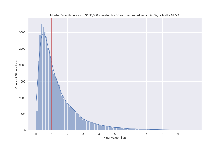
However run for 50,000 simulations and look at all 50,000 results.
The notebook accompanying this post contains code that creates a 50,000 row X 30 column matrix of results, transposes this into 30 Row X 50,000 column pandas DataFrame. Each column represents one of the 50,000 simulations, each row the value at the end of each year.
The head and tail of the first 5 columns of this DataFrame are shown below

Examine the results
The last row of this DataFrame, row 29, contains the final result of the investment for each of the 50,000 simulations. Using the pandas.describe() method to look at some summary statistics will output
count       50,000.00
mean     1,504,838.27
std      1,700,290.69
min         11,131.75
25%        514,762.68
50%        980,789.64
75%      1,848,145.76
max     37,897,980.93
Note the following
- The standard deviation is extremely large
- The mean 1,504,838.27 is remarkably close to the amount guaranteed using a deterministic approach which calculated final value of 1,522,031.27.
- The minimum value is extremely poor – 11,131,75 – however this is highly unlikely
- The maximum value is spectacular – 37,897,980 although equally unlikely.
- Half of the returns, between the 25th and 75th percentiles, were in the range 514,762 and 1,848,145
- The median is considerably less than the mean – this is a characteristic of a lognormal distribution.
A plot of the distribution is shown below – the red line is the portfolio at the 50th percentile.
Make some statements
percentiles = [1,5,10]
v99,v95,v90 = np.percentile(final_year, percentiles)

print(f'There is a 99% chance that the investment will be at least {v99:,.0f} at maturity')
print(f'There is a 95% chance that the investment will be at least {v95:,.0f} at maturity')
print(f'There is a 90% chance that the investment will be at least {v90:,.0f} at maturity')

There is a 99% chance that the investment will be at least 94,828 at maturity.
There is a 95% chance that the investment will be at least 195,235 at maturity.
There is a 90% chance that the investment will be at least 282,166 at maturity.
Using Monte Carlo to Calculate Value At Risk (VaR)
VaR is a measurement of the downside risk of a position based on the current value of a portfolio or security, the expected volatility and a time frame. It is most commonly used to determine both the probability and the extent of potential losses. There are several different ways to calculate VaR, this approach uses a parametric Monte Carlo method.
For more information on Var see Investopedia https://www.investopedia.com/terms/v/var.asp.
VaR allows investors to make statements such as “there is a 95% chance that the investment will be at least $50,000 in 1 months time”.
A common problem with VaR is when expected volatility is underestimated, for example black swan events such as the financial crisis of 2008, the lockdown of 2020 etc.
VaR is generally used for short time horizons, rarely if ever stretching past 1 year.
For example
An investor has $100,000 to invest and would like to know with 95% confidence what are the potential losses in 1 months time. Assuming 21 days / month.
Deterministic Approach
A very simple calculation with the code shown below. The 2 points to note are
1 – Volatility is proportional to the square root of time hence vol * np.sqrt(t/TRADING_DAYS) – See here for an explanation why this is so.
2 – I am using a percent point function from scipy.stats.nomal distribution module to calculate VaR.
CL = 0.95
pv = 100000
vol = 0.185
t = 21
TRADING_DAYS = 252

from scipy.stats import norm

cutoff = norm.ppf(CL)
VaR = (pv) * vol * np.sqrt(t/TRADING_DAYS) * cutoff

print("At {:.2f} confidence level, loss will not exceed {:,.2f}".format(CL, VaR))
print("This represents a move of {:.2f} standard deviations below the expected return".format(cutoff))

At 0.95 confidence level, loss will not exceed 8,784.32
This represents a move of 1.64 standard deviations below the expected return
In the accompanying Jupyter Notebook, I have refactored the above code into a simple function deterministic_VaR(pv, vol, T, CL)
Non-Deterministic Approach
To spice things up a little, we can use the yfinance package to download some real stock prices and try this out.
An investor wishes to buy $100,000 TSLA shares, what is the VaR after 21 days?.
The code downloads the Adjusted Close and calculates the log returns. Volatility is modelled as the standard deviation of log returns and annualised by multiply standard deviation by the square root of time.
# Latest Price
prices = yf.download(tickers=ticker, start=start, end=end)[['Adj Close']].copy()

# Log returns
prices['Log Rets'] = np.log(prices['Adj Close'] / prices['Adj Close'].shift(1))

# Dailty std
daily_vol = np.std(prices['Log Rets'])

# Annualized Volatility
vol = daily_vol * TRADING_DAYS ** 0.5
At the time of writing, the annualised volatility of TSLA was 54%.
Latest Price and Expected Return
Assume expected return 25% / year however due to the relatively short term nature of Var (here 21 days) the effect of expected return on VaR is negligible.
A simple function to run the simulation
def MC_VaR(pv, er, vol, T, iterations):

    end = pv * np.exp((er - .5 * vol ** 2) * T +
                     vol * np.sqrt(T) * np.random.standard_normal(iterations))

    ending_values = end - pv

    return ending_values

iterations = 50000

at_risk = MC_VaR(pv=value, er=er, vol=vol, T=t/TRADING_DAYS, iterations=iterations)

at_risk
The variable at_risk is a simple numpy.array, an example of which would look like
array([-21173.92356515,  -8577.34023718,   8736.59805928, ...,
        -1919.90496093, -15499.64852872,  18248.69214789])
Display the distribution
The distribution of possible losses and gains over this month.
The red, blue and green verticals are the VaR at confidence levels 99%, 95% and 90% respectively.

Compare deterministic and non-deterministic methods
For example
With confidence levels of 99%, 95% and 90% what are the maximum losses for TSLA
Deterministic
v99 = deterministic_VaR(pv=value, vol=vol, T = t/TRADING_DAYS, CL = 0.99)
v95 = deterministic_VaR(pv=value, vol=vol, T = t/TRADING_DAYS, CL = 0.95)
v90 = deterministic_VaR(pv=value, vol=vol, T = t/TRADING_DAYS, CL = 0.90)
At 99% confidence level, loss will not exceed 36,422.21
At 95% confidence level, loss will not exceed 25,752.47
At 90% confidence level, loss will not exceed 20,064.47
Non Deterministic
percentiles = [1,5,10]
v99,v95,v90 = np.percentile(at_risk, percentiles) * -1
At 99% confidence level, loss will not exceed 29,987.63
At 95% confidence level, loss will not exceed 21,955.62
At 90% confidence level, loss will not exceed 17,393.15
Summary
This is not the only method to calculate VaR – this method is known as a parameterised calculation of VaR, using an underlying distribution that I think the stock market will follow. Other investors disagree, and instead may use a different distribution, for example lognormal, Bernoulli distributions. Other analysts may take an empirical view and construct their own heuristic based distribution.
If anyone with needs assistance with Data Science, Data Engineering or Python problems please get in touch with our new Data Science professional services group.
Share this: